2
$\begingroup$

Am trying to find a function that could fit this data for bond breaking minimum path but so far haven't found one. I have previously fitted such data to Fourier series using NonlinearModelFit but had trouble fitting this one. I would greatly appreciate your help.

data1={{-4.238, 0.027},{-4.137, 0.394},{-3.95, 2.048},{-3.808, 4.175},{-3.69, 6.485},{-3.547, 10.003},{-3.444, 12.996},{-3.267, 19.061},{-3.128, 24.549},{-2.986, 30.771},{-2.873, 36.075},{-2.71, 44.056},{-2.545, 52.326},{-2.386, 60.124},{-2.231, 67.266},{-2.067, 74.144},{-1.902, 80.393},{-1.777, 84.856},{-1.615, 90.527},{-1.465, 95.936},{-1.332, 100.951},{-1.219, 105.414},{-1.111, 109.93},{-1.032, 113.396},{-0.943, 117.439},{-0.858, 121.535},{-0.788, 125.158},{-0.714, 129.201},{-0.654, 132.719},{-0.598, 136.159},{-0.494, 143.116},{-0.433, 147.422},{-0.395, 150.126},{-0.294, 157.136},{-0.226, 161.363},{-0.171, 164.278},{-0.108, 166.798},{0.02, 168.584},{0.144, 164.987},{0.191, 162.072},{0.251, 157.215},{0.312, 150.914},{0.372, 143.615},{0.49, 126.366},{0.525, 120.668},{0.569, 113.474},{0.62, 104.994},{0.68, 94.886},{0.724, 87.718},{0.79, 77.531},{0.834, 71.283},{0.888, 64.141},{0.967, 54.794},{1.024, 48.782},{1.08, 43.452},{1.147, 37.519},{1.22, 31.585},{1.306, 25.389},{1.372, 21.031},{1.465, 15.386},{1.576, 9.321},{1.673, 4.464},{1.784, -0.656},{1.91, -6.012},{2.052, -11.421},{2.211, -16.855},{2.372, -21.818},{2.542, -26.622},{2.715, -31.243},{2.949, -37.439},{3.086, -41.273},{3.296, -47.469},{3.457, -52.562},{3.772, -63.038},{3.888, -66.924},{4.103, -74.091},{4.257, -79.08}}

Here is my code

fit = NonlinearModelFit[data1,
  A + Μ Cos[x] + Ν Cos[2 x] + Ξ Cos[3 x] + Ο Sin[x] + Π Sin[2 x] + Ρ Sin[3 x] +  Σ Sin[4 x], 
  {{A, 150}, {Μ, 3}, {Ν, 1}, {Ξ, 1}, {Ο, 1}, {Π, 1}, {Ρ, 1}, {Σ, 1}}, x,
   ConfidenceLevel -> 0.99, MaxIterations -> 1000, Method -> Automatic]
fitplot = 
 Show[ListPlot[data1, PlotMarkers -> O , PlotStyle -> Red], 
  Plot[Normal[fit], {x, -4, 4},
   AxesLabel -> {"Reaction Coordinate", 
     "Energy/\!\(\*SuperscriptBox[\(kcalmol\), \(-1\)]\)"}, 
   PlotStyle -> Blue], Frame -> True, Axes -> False]

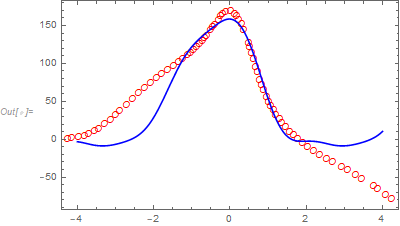
data and fit

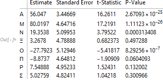
fit["ParameterTable"]

Parameter table from fit

(*assigning the equation of the fitted parameters to a function V[x] *)
V[x_?NumericQ] := fit[x]
$\endgroup$
1
  • $\begingroup$ But why do you fit with Fourier series, is there any reason to expect a periodic function? $\endgroup$
    – yarchik
    Commented Jun 2, 2020 at 16:35

3 Answers 3

6
$\begingroup$

Of course, a better fit could be obtained if you increased the number of parameters (within reason! a model with too many parameters will fit anything). To make it easier to explore that, let's use indexed variables as the multiplicative factors and generate the model and parameter list automatically, as a function of the number of components $n$ we want to include:

With[{n = 5},
  fit = NonlinearModelFit[
    data1,
    Total[{Table[a[i] Cos[i omega x], {i, 0, n}], Table[b[i] Sin[i omega x], {i, 0, n}]}, 2],
    Flatten@{Array[a, n + 1, 0], Array[b, n], omega}, x, 
    Method -> "NMinimize"]
  ];

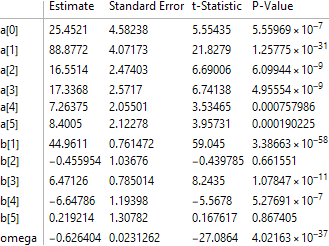
fit["ParameterTable"]

Plot[
  fit[x], {x, data1[[1, 1]], data1[[-1, 1]]},
  PlotStyle -> Red,
  Prolog -> {PointSize[0.01], Black, Point[data1]}
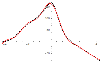
]

table of parameters from the fit

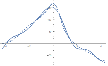
plot of fit (line) and data (points)

$\endgroup$
3
  • $\begingroup$ Very nice solution! It is quite good with n=5 (as you show) and with n=7, the computed and points are nearly perfect. $\endgroup$
    – Mark R
    Commented Jun 2, 2020 at 19:38
  • $\begingroup$ @MarkR Yes the fit will get better and better the more parameters you introduce, until you have as many parameters as you have points, and then you will just be interpolating your function :-) Beware of overfitting! $\endgroup$
    – MarcoB
    Commented Jun 2, 2020 at 19:44
  • $\begingroup$ thanks for the warning. $\endgroup$
    – Mark R
    Commented Jun 4, 2020 at 20:10
4
$\begingroup$

In your "Fourieranalysis" it's necessary to include the frequency ω as an additional parameter!

Try

fit = NonlinearModelFit[
         data1, 
         A + Μ Cos[ω x] + Ν Cos[2 ω x] + Ξ Cos[3 ω x] + 
           Ο Sin[ω x] + Π Sin[2 ω x] + ΡSin[3 ω x] + Σ Sin[4 ω x],
         {A, Μ, Ν, Ξ, Ο, Π,Ρ, Σ, ω },
         x, Method -> "NMinimize"]

Show[{
  Plot[Normal[fit], {x, -data1[[1, 1]], data1[[-1, 1]]}], 
  ListPlot[data1]},
 PlotRange -> All]

plots with fit

$\endgroup$
4
  • $\begingroup$ Rather than Normal[fit], it may be more natural to use fit[x] inside the plot. Also, I am not sure that there should be a negative sign in -data[[1, 1]]: shouldn't that be just data[[1, 1]]? $\endgroup$
    – MarcoB
    Commented Jun 2, 2020 at 15:33
  • $\begingroup$ @MarcoB Your are right Fit[x] look more natural here. For the Plot, I just specified the range explicitly but in this case it should be just data1[[1,1]] $\endgroup$
    – fred85
    Commented Jun 2, 2020 at 16:11
  • $\begingroup$ @ UIrich Neumann I had tried adding frequency but the fit wasn't that good. Here I just want an analytical expression which fits the data regardless of the form. I would use these expression in the NIntegrate to calculate several integrals along the energy axis as shown here $\endgroup$
    – fred85
    Commented Jun 2, 2020 at 16:23
  • $\begingroup$ @fred85 The fit with frequency in MarcoB 's and my answer is quite good I think. $\endgroup$ Commented Jun 2, 2020 at 17:35
3
$\begingroup$

This is just an extended comment to add to the approaches that @MarcoB and @UlrichNeumann provided.

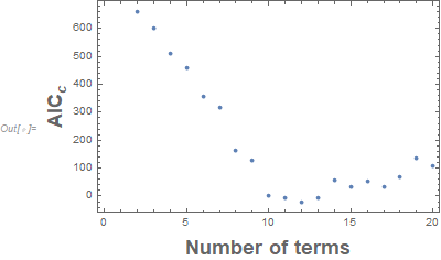
To determine how many sets of cosine/sine terms are appropriate one needs a metric to judge the quality of the resulting model. A common statistical metric is $AIC_c$ which is available from NonlinearModelFit. $AIC_c$ is a relative measure and allows you to rank competing models. The model with the smallest $AIC_c$ value gives you the best of a collection of horrible or very good models.

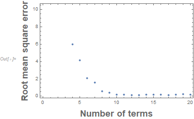
An alternative approach is to use the root mean square error: fit["EstimatedVariance"]^0.5. This is an "absolute" measure which gives you the standard error of the prediction at the mean of the predictor values. One uses their subject matter knowledge to decide on if a model's root mean square error is small enough.

For this dataset the following figures for $AIC_c$ and root mean square error can be generated:

results = {{2, 659.943, 16.5092}, {3, 599.761, 10.9489}, {4, 510.368, 5.99449},
   {5, 457.662, 4.15564}, {6, 357.128, 2.10662}, {7, 316.324, 1.56969},
   {8, 163.249, 0.562518}, {9, 128.91, 0.434393}, {10, 1.10447, 0.18216},
   {11, -5.198, 0.167454}, {12, -20.9262, 0.144134}, {13, -5.81008, 0.15079},
   {14, 57.7525, 0.214809}, {15, 32.834, 0.171122}, {16, 51.2808, 0.179277},
   {17, 33.2177, 0.146872}, {18, 68.3095, 0.168188}, {19, 134.711, 
    0.233195},
   {20, 110.034, 0.176447}};
ListPlot[results[[All, {1, 2}]], Frame -> True,
 FrameLabel -> (Style[#, Bold, 18] &) /@ {"Number of terms", 
    "\!\(\*SubscriptBox[\(AIC\), \(c\)]\)"}]
ListPlot[results[[All, {1, 3}]], Frame -> True,
 FrameLabel -> (Style[#, Bold, 18] &) /@ {"Number of terms", 
    "Root mean square error"}]

AICc vs number of terms

Root mean square error vs number of terms

So $AIC_c$ suggests that having 12 terms is the best of the models with 2 to 20 sets of terms and 12 terms also has the minimum root mean square error.

If one picked 12 terms based on those results, that would be doing so without any subject matter knowledge. And that would seem nuts to me.

If a mean square error of 0.562518 associated with 8 terms is adequate for you, then based on your knowledge, that's what you should choose. There is no law that says you need to choose the model with the miniminum $AIC_c$ or the minimum root mean square error. While both of those statistics are good guides as to what your data supports, you need to use your subject matter knowledge to decide. You need to choose an "adequate" model by your standards.

$\endgroup$
3
  • $\begingroup$ Thank you. AIC looks interesting and I will definitely read more about it. However, what am looking for is any analytical expression that fits the data. Such expression with be passed to an NIntegrate. $\endgroup$
    – fred85
    Commented Jun 2, 2020 at 16:56
  • $\begingroup$ AIC simply ranks the models. And then you pick the desired model. AIC does not change the model in any way. So you end up with an analytical expression as desired. But note that some use AIC in a weighting scheme and "average" the models examined (called "model averaging"). I don't recommend that in this case. $\endgroup$
    – JimB
    Commented Jun 2, 2020 at 18:13
  • $\begingroup$ I think it is really useful in evaluating the number of parameters one might need to effectively fit a certain model. I have fit the model proposed by @MarcoB with n=6 as you suggested and it fits very well. Thanks for mentioning it here. $\endgroup$
    – fred85
    Commented Jun 2, 2020 at 18:23

Your Answer

By clicking “Post Your Answer”, you agree to our terms of service and acknowledge you have read our privacy policy.

Not the answer you're looking for? Browse other questions tagged or ask your own question.