two weeks ago, I post a question see, and I got its answer, however, I would like to vary the values: g from (0.02 to 0.07), R from (0.1 to 0.3),and k2 from (0.03 to 0.07) by an increment of 0.01 using for Do loop. Can you please help?
$\begingroup$
$\endgroup$
6
-
$\begingroup$ And what do you need to get out of the loop? $\endgroup$– Alex TrounevCommented Sep 28, 2018 at 3:22
-
$\begingroup$ I want to see the behavior of y' and y? $\endgroup$– aluuzzCommented Sep 28, 2018 at 4:38
-
$\begingroup$ How do you want to visualize data - on a plane or in space? $\endgroup$– Alex TrounevCommented Sep 28, 2018 at 5:30
-
$\begingroup$ I want to visualize data on a plane. $\endgroup$– aluuzzCommented Sep 28, 2018 at 5:36
-
$\begingroup$ A set of curves on one plane or each curve on one plane? $\endgroup$– Alex TrounevCommented Sep 28, 2018 at 5:46
|
Show 1 more comment
1 Answer
$\begingroup$
$\endgroup$
3
It is possible to use the following model for parametric studies.
p[Z0_, g0_, k0_, R0_] := Block[{Z = Z0, g = Rationalize[g0, 0],
       k2 = Rationalize[k0, 0],
       \[Epsilon] = 10^-4, R = Rationalize[R0, 0]},
      ps = ParametricNDSolveValue[{y''[r] + 2 y'[r]/r == k2 Sinh[y[r]],
         y[\[Epsilon]] == y0, y'[\[Epsilon]] == 0,
         WhenEvent[r == 1, y'[r] -> y'[r] + Z g]}, {y,
         y'}, {r, \[Epsilon], R}, {y0}, Method -> "StiffnessSwitching",
        WorkingPrecision -> 20];
      sol = FindRoot[Last[ps[y0]][R], {y0, -1},
         Evaluated -> False][[1, 2]];
      Plot[First[ps[sol]][r], {r, \[Epsilon], R}, AxesLabel -> {r, y},
       PlotLabel ->
        Grid[{{"Z", "g", "k2", "R"}, {Z0, g0, k0, R0}}, Frame -> All]]]

    p1[Z0_, g0_, k0_, R0_] := Block[{Z = Z0, g = Rationalize[g0, 0],
       k2 = Rationalize[k0, 0],
       \[Epsilon] = 10^-4, R = Rationalize[R0, 0]},
      ps = ParametricNDSolveValue[{y''[r] + 2 y'[r]/r == k2 Sinh[y[r]],
         y[\[Epsilon]] == y0, y'[\[Epsilon]] == 0,
         WhenEvent[r == 1, y'[r] -> y'[r] + Z g]}, {y,
         y'}, {r, \[Epsilon], R}, {y0}, Method -> "StiffnessSwitching",
        WorkingPrecision -> 20];
      sol = FindRoot[Last[ps[y0]][R], {y0, -1},
         Evaluated -> False][[1, 2]];
      Plot[Last[ps[sol]][r], {r, \[Epsilon], R}, AxesLabel -> {r, y'},
       PlotLabel ->
        Grid[{{"Z", "g", "k2", "R"}, {Z0, g0, k0, R0}}, Frame -> All]]]
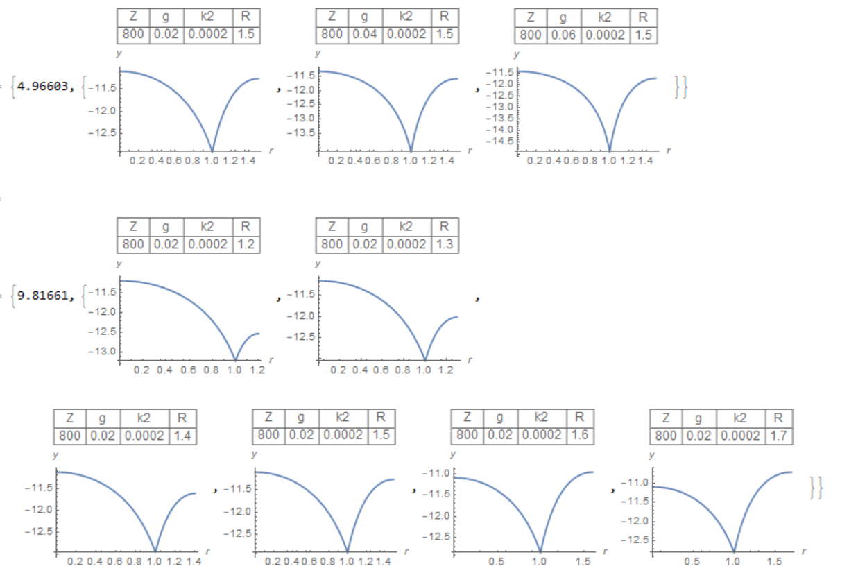
Two examples of using this code
Quiet[Table[
   p[800, g, 0.0002, 1.5], {g, 0.02, 0.06, .02}]] // AbsoluteTiming

Quiet[Table[
   p[800, .02, 0.0002, R], {R, 1.2, 1.7, .1}]] // AbsoluteTiming
-
$\begingroup$ Thank you so much, What is this method doing exactly? also, what is p1 and p ? $\endgroup$– aluuzzCommented Sep 28, 2018 at 17:02
-
$\begingroup$ Can I do this in one step 'Quiet[Table[ p[800, g, 0.0002, R], {g, 0.02, 0.06, .02}, {R, 1.2, 1.7, .1}]] // AbsoluteTiming' .? $\endgroup$– aluuzzCommented Sep 28, 2018 at 17:13
-
$\begingroup$ p and p1 are the figures y and y', respectively, as the solution of the problem with the selection of parameters indicated at the top of each of the figures. You can use tables with any combination of parameters, but I checked only two of them. $\endgroup$ Commented Sep 29, 2018 at 3:33

