Use of NDSolve in loops

Question

Im new to mathematica and have some problems to use NDSolve in a loop (at least i suspect this is the reason for my problems). I hope anybody can help me! Thanks a lot in advance! I created the following code block, which works just fine so far. But now i want to put the last code block into a loop and vary UL from 0 to 1.2 with steps of 0.1. I already tried it with a Do loop, but then i get loads of warnings such as 'ReplaceAll::reps: "{s} is neither a list of replacement rules nor a valid dispatch table, and so cannot be used for replacing'. I also tried it with a Table, but i couldn't the right syntax there too. At the end, i'd like to plot all the Un and j-Values against each other. How would you code this?

(*Input parameters*)
     UL = 0.8; nC = 0.00205498; nH = 0.0164398; nO = 0.00410996; nN = 0;
     Kp1 = 1.0853; Kp2 = 1.503*10^(9); ASRRU = (0.3/10000); p = 100000; 
     R = 8.3144598; h = 0.00055 ; T = 800 + 273; tau = 0.2; F = 96485.33289

(*Function*)
       nO2[x_] = ((2 nC + nH + nN) (2 nC - 4 Kp1 nC - nH - 2 x + 2 Kp1 x + \[Sqrt](8 (-1 + Kp1) nC (4 nC + nH -2 x) + ((6 - 4 Kp1) nC + nH + 2 (-1 + Kp1) x)^2))^2)/(2 Kp2^2 (2 nC - 4 Kp1 nC + nH - 2 Kp1 nH - 2 x + 2 Kp1 x + \[Sqrt](8 (-1 + Kp1) nC (4 nC + nH - 2 x) + ((6 - 4 Kp1) nC + nH + 2 (-1 + Kp1) x)^2))^2 p)

(*Codeblock for loop*)    
    s = NDSolve[{NO'[
         t] == (1/(2*F*
             ASRRU))*(((R*T)/(4*F)) (Log[0.21] - 
              Log[(nO2[NO[t]] *(R*T))/h]) - UL), NO[0] == nO}, 
      NO, {t, 0, 100}]
    Plot[Evaluate[NO[t] /. s], {t, 0, 1}, PlotRange -> All]
    Evaluate[NO[0.2] /. s]
    UN1[t_] = ((R*T)/(4*F)) (Log[0.21] - 
        Log[(nO2[Evaluate[NO[t] /. s]]*(R*T))/h])
    j[t_] = (UN1[t] - UL)/(ASRRU *10000)
    Un = NIntegrate[UN1[t], {t, 0, tau}]/tau
    J = NIntegrate[j[t], {t, 0, tau}]/tau

Answer 1

You don't actually need to put it in a loop. Mathematica has many other cleaner/faster/shorter ways of implementing this kind of thing. I'll give you three:

1. A Do loop (which you asked for, so it wouldn't be much of an answer if I didn't).
2. An alternative using Map (or /@), which shows up all over the place and is probably one of the most useful Mathematica functions.
3. A method using ParametricNDSolve, as suggested by @SjoerdSmit in comments, which is probably the way that a problem like this should be tackled.

A Do Loop

Here's a quick and dirty loopification of your code:

points = Last@Last@Reap@Do[
     s = NDSolve[{NO'[t] == 
         (1/(2*F*ASRRU))*(((R*T)/(4*F)) (Log[0.21] - Log[(nO2[NO[t]]*(R*T))/h]) - UL), 
       NO[0] == nO}, NO, {t, 0, 100}][[1, 1]];

     UN1[t_] = ((R*T)/(4*F)) (Log[0.21] - Log[(nO2[Evaluate[NO[t] /. s]]*(R*T))/h]);
     j[t_] = (UN1[t] - UL)/(ASRRU*10000);

     Sow[{NIntegrate[j[t], {t, 0, tau}]/tau, NIntegrate[UN1[t], {t, 0, tau}]/tau}],
    {UL, 0, 1.2, 0.1}]

ListPlot[points, AxesLabel -> {"j", "UN1"}]

All I've really done is put semicolons in, taken out your Plot, Flattened s, and added Sow and Reap to accumulate the results of the loop. It could definitely be improved, but I think that's something like what you were going for.

Using Map over a list of parameter values

Mathematica makes it nice and easy just use Map, or /@, and run everything over lists. (If you're not familiar with what f[#] & /@ list means, really check out the docs on Map and Function -- all it does is apply the function f to each element of list and give you back the transformed list).

To start off, get whatever range of parameters you're interested in:

ULrange = Range[0, 1.2, 0.1];

Then you can just Map your NDSolve over that:

s = NDSolve[{NO'[t] == 
    (1/(2*F*ASRRU))*(((R*T)/(4*F)) (Log[0.21] - Log[(nO2[NO[t]]*(R*T))/h]) - #), 
  NO[0] == nO}, NO, {t, 0, 100}][[1, 1]] & /@ ULrange;

In this case, s is now a vector of solutions for each of the different values of UL, as specified in ULrange. (Also, note the [[1, 1]]. There were a bunch of brackets { } cluttering up your solutions. NDSolve always gives lists, so it's sometimes nice just to pull out the one solution you're interested in.) You can have a look at these solutions by Mapping Plot over s:

Plot[Evaluate[NO[t] /. #], {t, 0, 1}, PlotRange -> All] & /@ s

Next, you can define your functions pretty much as before:

UN1[t_] = ((R*T)/(4*F)) (Log[0.21] - Log[(nO2[NO[t] /. #]*(R*T))/h]) & /@ s;
j[t_] = (UN1[t] - ULrange)/(ASRRU*10000);

where I've replaced NO[t] /. s with (NO[t] /. #) & /@ s, and the UL in j with ULrange. So both UN1 and j are now vector-valued functions:

Length /@ {UN1[t], j[t]}

(* {13, 13} *)

Finally, to get your points, just integrate:

points = Transpose@{NIntegrate[j[t], {t, 0, tau}]/tau, 
                  NIntegrate[UN1[t], {t, 0, tau}]/tau};

ListPlot[points, AxesLabel -> {"j", "UN1"}]

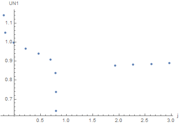
The Map and Do methods ultimately produce the same output, but there is no looping structure with Map. The main question is what you feel comfortable working with, and where your intuition can guide you best. However, nurturing your intuition for Map can only be a good thing.

Using ParametricNDSolve for a parameterized differential equation

I rarely think to use ParametricNDSolve (so thanks @SjoerdSmit), mainly because, on some level, I don't really believe that something this useful and easy could ever actually work. But it does!

Clear[UL]
sol = ParametricNDSolve[{NO'[t] == 
    (1/(2*F*ASRRU))*(((R*T)/(4*F)) (Log[0.21] - Log[(nO2[NO[t]]*(R*T))/h]) - UL), 
  NO[0] == nO}, NO, {t, 0, 100}, UL]

(* {NO -> ParametricFunction[ <> ]} *)

Then you can define UN1 and j as before, but with UL as a parameter:

UN1[UL_, t_] := ((R*T)/(4*F)) (Log[0.21] - Log[(nO2[Evaluate[NO[UL][t] /. sol]]*(R*T))/h])
j[UL_, t_] := (UN1[UL][t] - UL)/(ASRRU*10000)

Now you could just use ParametricPlot to get a pretty good picture of UN1 vs. j:

ParametricPlot[{NIntegrate[j[UL, t], {t, 0, tau}]/tau, 
  NIntegrate[UN1[UL, t], {t, 0, tau}]/tau}, {UL, 0, 1.2}]

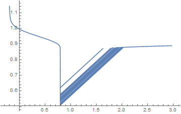
which nicely shows something weird going on. Be warned, though: that plot took over three minutes to plot, because it's having to do two NIntegrates for each point.

Alternatively, you could create some points (using Map again), and make a ListLinePlot:

points = {NIntegrate[j[#, t], {t, 0, tau}]/tau, 
    NIntegrate[UN1[#, t], {t, 0, tau}]/tau} & /@ Range[0, 1.2, 0.01]

ListLinePlot[points]

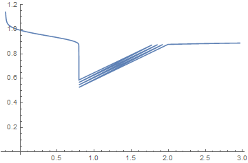
The beauty of this method (besides taking much less typing than the others) is that once you have your functions in terms of NO as a ParametricFunction, you have a whole lot more flexibility to play around with it without having to rederive everything.