Plotting for various parameter values with single code

Question

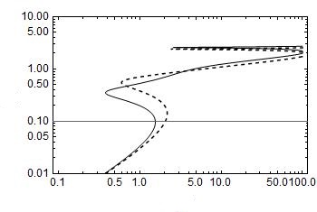
I am trying to plot for four different values of a parameter with the following code

axisFlip = # /. {x_Line | x_GraphicsComplex :> 
  MapAt[#~Reverse~2 &, x, 1], 
 x : ((PlotRange | FrameTicks) -> _) :> x~Reverse~2} &;
c = 0.1;
ω = -1.99;
v = -2.5;
y = 0.05;
s = v (1 + y);
q = v (1 - y);
a = 0;
ν = s - ω + ((
P*(1 - 2 δ*Cos[c] + δ^2))/(1 + 
  a*P *(1 - 2 δ*Cos[c] + δ^2)));
δ = q - ω + (P/(1 + a*P)) ;
LogLogPlot[{P Abs[(
1 + (ν - E^(I c)) (E^(I c) - δ))/(E^(I c) - 
  E^(-I c))]^2}, {P, 10^-2, 10^1}, PlotRange -> {10^-1, 10^2}, 
PlotPoints -> 100, ImageSize -> 350, Frame -> True, Axes -> True, 
FrameTicks -> {{{10^-2, 10^-1, 10^0, 10^1}, 
None}, {{10^-1, 10^0, 10^1, 10^2}, None}}, 
FrameStyle -> Directive[Black, FontSize -> 12]]

and

a1 = LogLogPlot[{P Abs[(
  1 + (ν - E^(I c)) (E^(I c) - δ))/(E^(I c) - 
    E^(-I c))]^2}, {P, 1/10^2, 10^1}, 
PlotStyle -> 
Directive[RGBColor[0., 0., 0.], AbsoluteThickness[1.48], Dashed], 
PlotRange -> {1/10, 10^2}, PlotPoints -> 100, ImageSize -> 350, 
Frame -> True, Axes -> True, 
FrameStyle -> Directive[Black, FontSize -> 12]] // axisFlip

Then in the same plot I want to add another variation in which I have to redefine $\nu$ and $\delta$ separately like

ν = q - ω + ((
P*(1 - 2 δ*Cos[c] + δ^2))/(1 + 
  a*P *(1 - 2 δ*Cos[c] + δ^2)));
δ = s - ω + (P/(1 + a*P)) ;

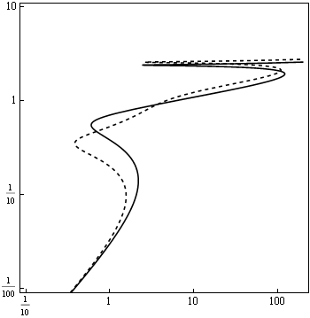
re-do the above process, generate another plot a2 with other parameters as before and then use g = Show[a1, a2] to get the desired output.

Is there a way to generate the output with a single code? Secondly, the Frame ticks are strange they should be $10^{-1},10^0,10^1,10^2$ on x-axis and $10^{-2},10^{-1},10^0,10^1$ on y-axis.

Answer 1

First, as good practice, limit the scope of your reclarations using With. Do not declare the variables you want to change, but use ReplaceRepeated to replace the variables with the intended value. Also, use indentation to make your code readable.

axisFlip = # /. {x_Line | x_GraphicsComplex :> MapAt[#~Reverse~2 &, x, 1], 
     x : ((PlotRange | FrameTicks) -> _) :> x~Reverse~2} &;
With[
 {c = 0.1, ω = -1.99, v = -2.5, y = 0.05, a = 0},
 With[
  {s = v (1 + y), q = v (1 - y)},
  LogLogPlot[
    Evaluate@ReplaceRepeated[
      P Abs[(1 + (ν - E^(I c)) (E^(I c) - δ))/(E^(I c) - E^(-I c))]^2
      , {
       {
        ν -> s - ω + ((P*(1 - 2 δ*Cos[c] + δ^2))/(1 + a*P*(1 - 2 δ*Cos[c] + δ^2))),
        δ -> q - ω + (P/(1 + a*P))
        },
       {
        ν -> q - ω + ((P*(1 - 2 δ*Cos[c] + δ^2))/(1 + a*P*(1 - 2 δ*Cos[c] + δ^2))),
        δ -> s - ω + (P/(1 + a*P))
        }
       }
      ]
    , {P, 0.009, 11.}
    , AspectRatio -> 1
    , PlotRange -> {0.1, 2 100}
    , PlotTheme -> "Scientific"
    , PlotStyle -> {Black, Directive[Black, Dashed]}
    , ImageSize -> 350
    , FrameStyle -> Directive[Black, FontSize -> 12]
    , FrameTicks -> {{PowerRange[10^-2, 10^2], 
       None}, {PowerRange[10^-2, 10^2], None}}
    ] // axisFlip
  ]]