6
$\begingroup$

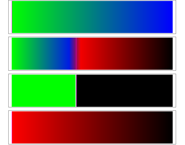
I've recently been playing around with ColorFunction and have run into a small snag. I'm ultimately looking to apply combinations of color schemes to the same data set. In the code below (simplified example), I want red for x < 0.4 and blue above.

line[x0_] := Line[{{x0, 0}, {x0, 0.2}}];
graphic[x0_, colorfunc_] := 
  DensityPlot[x, {x, 0, 1}, {y, 0, .2}, 
    AspectRatio -> Automatic, 
    Frame -> True, FrameTicks -> None, 
    ColorFunction -> (colorfunc &), 
    Epilog -> {Green, line[x0]}]
GraphicsColumn[
  {graphic[0.4, If[# < 0.4, RGBColor[1, 0, 0], RGBColor[1, 1, 1]]],
   graphic[0.4, If[# > 0.4, RGBColor[1, 0, 0], RGBColor[0, 0, 1]]],
   graphic[0.4, If[# > 0.4, RGBColor[0, 0, 1], RGBColor[1, 1, 1]]]}, 
  ImageSize -> 600]

enter image description here

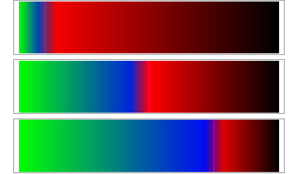
I'm curious as to why the boundaries seem so diffuse - I was looking for the output to look more along the lines of the following, with hard boundaries.

enter image description here

Is there something I'm missing that causes this behavior?

EDIT:

I originally started digging into this while playing around with Colorize, so the discontinuity that appears around x0 from m_goldberg's response would be worrisome.

graphic2[x0_, colorfunc_] := 
  DensityPlot[UnitStep[x - x0], {x, 0, 1}, {y, 0, .2}, 
  AspectRatio -> Automatic, Frame -> True, FrameTicks -> None, 
  ColorFunction -> (colorfunc &), Epilog -> {Magenta, line[x0]}]

funcA[f_] := RGBColor[0, 1 - f, f];
funcB[f_] := RGBColor[1 - f, 0, 0];
funcAB[f_, x0_] := If[f < x0, funcA[f/x0], funcB[(f - x0)/(1 - x0)]];

GraphicsColumn[{
  graphic[0, funcA[#]],
  graphic[0.4, funcAB[#, 0.4]],
  graphic2[0.4, funcAB[#, 0.4]],
  graphic[0, funcB[#]]
  }]

enter image description here

So, perhaps a more accurate descriptor of what I'm looking at would be, how do I generate a custom 'composite' palette from existing gradients, with sharp boundaries?

enter image description here

The blending isn't necessarily the worst thing in the world (and certainly isn't without merit...), but in my mind that can (ie should) be incorporated by having the constituents overlap a designated amount.

$\endgroup$
2

4 Answers 4

2
$\begingroup$

Update: The second approach with Show can be extended easily to more than two regions without having to worry about scaling of the color functions by making the two arguments a list of thresholds of length n>=1 and a list of color functions of length n + 1, respectively.

ClearAll[graphic5]
graphic5[x0 : {__}, colorfuncs : {__}, o : OptionsPattern[]] := 
 Show[DensityPlot[x, {x, #[[1]], #[[2]]}, {y, 0, .2}, 
     AspectRatio -> Automatic, Frame -> True, FrameTicks -> None, 
     ColorFunction -> #2, GridLines -> {x0, None}, 
     ImagePadding -> Scaled[.005],  PlotRangePadding -> .01, 
     AspectRatio -> 1/12, GridLinesStyle -> Directive[Thick, White], 
     Method -> {"GridLinesInFront" -> True}] & @@@ 
   Transpose[{Partition[Flatten[{0, x0, 1}], 2, 1], colorfuncs}], 
  PlotRange -> All, o]

Examples:

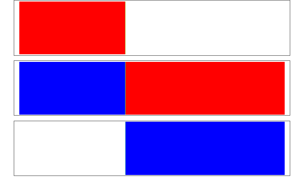
graphic5[{.4, .7}, {"TemperatureMap", Cyan &, "Rainbow"}]

enter image description here

graphic5[{.3, .4, .8}, {"TemperatureMap", Green &, "DeepSeaColors", 
  ColorData[{"Rainbow", "Reverse"}]}, AspectRatio -> 1/12, Frame -> False]

enter image description here

Original answer:

Two methods, the first one graphic3 uses @m_goldberg's idea of introducing a jump in the input function, and the second uses Show to combine two plots each with its own color function:

ClearAll[graphic3, graphic4]
graphic3[jump_: 1][x0_, colorfunc_] := DensityPlot[
  Piecewise[{{x, x <= x0}, {jump + x, x >= x0}}], 
  {x, 0, 1}, {y,  0, .2}, 
  AspectRatio -> Automatic, Frame -> True, 
  FrameTicks -> None, ImagePadding -> 1, PlotPoints -> 100, 
  ColorFunctionScaling -> False, ColorFunction -> (colorfunc &), 
  Epilog -> {White, line[x0]}]

funcA[f_] := RGBColor[0, 1 - f, f];
funcB[f_] := RGBColor[1 - f, 0, 0];
funcAB2[jump_: 1][f_, x0_] := If[f <= x0, funcA[f/x0], funcB[(f - jump - x0)/(1 - x0)]];

graphic3[][x0, funcAB2[][#, x0]]

enter image description here

graphic3[2][x0, If[# <= x0, Green, ColorData["TemperatureMap"][(# - 2 - x0)/(1 - x0)]]]

enter image description here

graphic4[x0_, colorfunc : {_, _}] := Show[DensityPlot[x, {x, #[[1]], #[[2]]}, {y, 0, .2}, 
     AspectRatio -> Automatic, Frame -> True, FrameTicks -> None, 
     ColorFunction -> (colorfunc[[#2]]), 
     Epilog -> {White, line[x0]}] & @@@ {{{0, x0}, 1}, {{x0, 1}, 2}}, 
  PlotRange -> All, ImagePadding -> 1]

graphic4[.4, {funcA, funcB}]

enter image description here

graphic4[.4, {Green &, "TemperatureMap"}]

enter image description here

$\endgroup$
2
$\begingroup$

tl;dr Mathematica detects discontinuities in the function you plot, but not in the colour function. Add an exclusion manually using Exclusions -> (x == 0.4).


The reason why you see this is that the sampling of the function must necessarily be discrete. There may not be a sampling point just at 0.4, where you want the break. Imagine that there is one at 0.3 (blue) and one at 0.5 (red). DensityPlot (and generally, all functions that produce coloured polygons) will interpolate between these two linearly. This interpolation is done by the graphics rendering component, not by the plotting one. It can also cause trouble with colour functions like "Rainbow", which change smoothly through many colours, e.g. purple-blue-green-yellow-red. If the function you plot varies quickly and jumps straight from purple to yellow, then the interpolation between the two won't produce any blue or green: it interpolates between colours, not between function values.

@m_goldberg suggests you use UnitStep, and it does indeed work well with that function. Why? Because Mathematica detects the discontinuity in UnitStep and places a sampling point just before 0.4 and another one just after 0.4. Furthermore, it leaves a gap between them instead of interpolating smoothly.

This automatical detection of discontinuities is called exclusion detection in Mathematica, and is controlled by the Exclusions option. You can specify exclusions manually.

Thus, all you need to do is add the option Exclusions -> (x == 0.4) to DensityPlot.

$\endgroup$
1
$\begingroup$

There is nothing wrong with your color function, but you need change the definition of you density function.

line[x0_] := Line[{{x0, 0}, {x0, 0.2}}];
graphic[x0_, colorfunc_] :=
  DensityPlot[UnitStep[x - x0], {x, 0, 1}, {y, 0, .2},
    AspectRatio -> Automatic,
    Frame -> True, FrameTicks -> None,
    ColorFunction -> (colorfunc &),
    Epilog -> {Green, line[x0]}]
graphic[0.4, If[# > 0.4, RGBColor[1, 0, 0], RGBColor[0, 0, 1]]]

plot

$\endgroup$
1
  • $\begingroup$ Thank you for your response! Unfortunately that fix doesn't work for me - I'm looking for the constituent sections to be variable themselves, something the UnitStep strips away. More info edited into the question. $\endgroup$
    – stallada
    Commented Jun 6, 2018 at 20:14
0
$\begingroup$

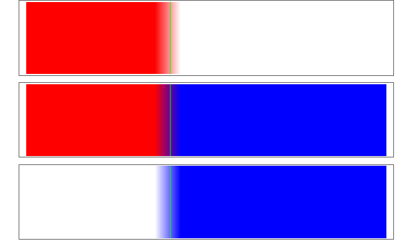
Szabolcs explains why this happens, but another solution is simply brute force through dense sampling, by way of PlotPoints. Adding only PlotPoints -> 300 to your code gives this output:

enter image description here

$\endgroup$

Your Answer

By clicking “Post Your Answer”, you agree to our terms of service and acknowledge you have read our privacy policy.

Not the answer you're looking for? Browse other questions tagged or ask your own question.