Function with EllipticK does not evaluate in certain range

Question

I have some rather complicated function (related to the capacitance of coplanar waveguides for specific geometric parameters, for those who are interested) which I've trimmed down to the following for simplicity:

SampleFun[w_, s_, g_, h2_] := Module[{a, b, c0, k2, k2p, k4, k4p, q2},
  a = s/2;
  b = s/2 + w;
  c0 = g + w + s/2;
  k2 = a/b*Sqrt[(1 - b^2/c0^2)/(1 - a^2/c0^2)];
  k2p = Sqrt[1 - k2^2];
  k4 = Sinh[Pi*a/2/h2]/Sinh[Pi*b/2/h2]*
    Sqrt[(1 - Sinh[Pi*b/2/h2]^2/Sinh[Pi*c0/2/h2]^2)/(
     1 - Sinh[Pi*a/2/h2]^2/Sinh[Pi*c0/2/h2]^2)];
  k4p = Sqrt[1 - k4^2];
  q2 = EllipticK[k4]/EllipticK[k4p]*1/2*EllipticK[k2p]/EllipticK[k2];
  Return[q2]]

The source of the equation is a combination of theory found in Gevorgian et al (1995) (fairly legible) and Garg et al (1979) around p. 376. In its entire form it will give the capacitance per unit length of a coplanar waveguide resonator with finite ground planes and a double layered substrate of finite thicknesses.

Now, since this function depends sensitively on the geometric input parameters, lets say that we can always take w = 1500*10^-9, s = 30*10^-6, g = 50*10^-6, and h2 is a number that goes from 0 (lets take 0.1*10^-9 as we can't divide by 0) to 400*10^-9 for the range that I am interested in.

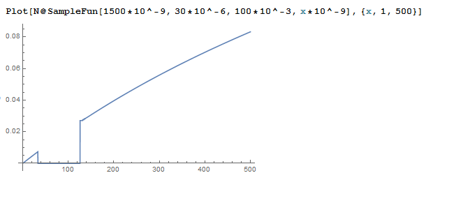
If we look at the function in this range, then it behaves in a peculiar way; for low values there seems to be an error in the calculation, and it gives exactly 0.

Does anyone understand what is going on here, and how I could go about fixing it? I believe the problem stems from the EllipticK[k4p] part, as the rest seems to evaluate nicely, but it might be a combination of factors so I didn't leave out more. It is quite problematic for my calculation, as h2 is approximately 100*10^-9 in the geometry I am considering, which falls exactly in this gap.

Note, this is for Mathematica 10.0.2, which now that I write it I should definitely update as it might be something that is fixed in future versions.

Answer 1

It is unfortunate that the OP neglected to give a source for the formula (always give references if providing an unfamiliar formula!) in the question; I will nevertheless proceed with my guess, based on a cursory look at the provided code.

The heart of the issue seems to be about the OP neglecting to check if his/her preferred convention for elliptic integrals matches with Mathematica's preferred convention. I have ranted about this in this math.SE post, but suffice it to say that the OP's formula seems to be assuming the modulus $k$ to be the argument, while EllipticK[] needs the parameter $m$ as an argument.

Thus:

SampleFun[w_, s_, g_, h2_] := Module[{a, b, c0, m2, m2p, m4, m4p},
      a = s/2; b = s/2 + w; c0 = g + w + s/2;
      m2 = (a/b)^2 (1 - b^2/c0^2)/(1 - a^2/c0^2);
      m2p = 1 - m2;
      m4 = (Sinh[π a/2/h2]/Sinh[π b/2/h2])^2
           (1 - Sinh[π b/2/h2]^2/Sinh[π c0/2/h2]^2)/
           (1 - Sinh[π a/2/h2]^2/Sinh[π c0/2/h2]^2);
      m4p = 1 - m4;
      EllipticK[m4]/EllipticK[m4p]*1/2*EllipticK[m2p]/EllipticK[m2]]

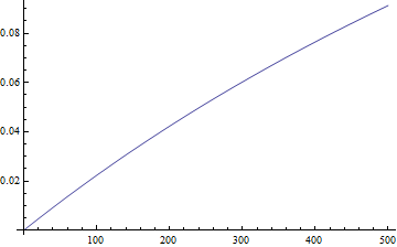
Plot[SampleFun[15*^-7, 3*^-5, 1/10, x 1*^-9], {x, 1, 500}, WorkingPrecision -> 30]

---

Here is the long-overdue follow-through. The key insight here is that one can use the relationship between the complete elliptic integral of the first kind and the arithmetic-geometric mean, after which one can then use the homogeneity relation for the AGM to stave off cancellations and bad scaling. Applying this to the specific problem here, we have the following stabilized routine:

SampleFun[w_, s_, g_, h2_] := Module[{a, b, c0, ab, ac0, bc0, sab, sac0, sbc0},
      a = s/2; b = s/2 + w; c0 = g + w + s/2;
      ab = a/b; ac0 = 1 - (a/c0)^2; bc0 = 1 - (b/c0)^2;
      sab = Sinh[π a/2/h2]/Sinh[π b/2/h2];
      sac0 = 1 - (Sinh[π a/2/h2]/Sinh[π c0/2/h2])^2;
      sbc0 = 1 - (Sinh[π b/2/h2]/Sinh[π c0/2/h2])^2;

      1/2 * ArithmeticGeometricMean[Sqrt[sac0], sab Sqrt[sbc0]]/
      ArithmeticGeometricMean[Sqrt[sac0], Sqrt[sac0 - sab^2 sbc0]] *
      ArithmeticGeometricMean[Sqrt[ac0], Sqrt[ac0 - ab^2 bc0]]/
      ArithmeticGeometricMean[Sqrt[ac0], ab Sqrt[bc0]]]

which is now much less prone to subtractive cancellation or overflow than the previous version. (Try using it in the Plot[] command above without the WorkingPrecision option set.)