Problem plotting partial sum of a Fourier series

Question

I'm new to using Mathematica, and I have a problem with plotting Fourier series partial sums.

In particular, my target is

1. to plot the Fourier series of my piecewise function and with that function on a single plot

2. and then to compare the genereted trigonometric polynomial with the original function to find point where they are closest to each other.

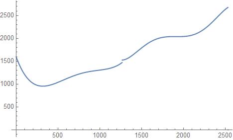
I started with this piecewise function which was generated by a previous fitting of my data.

f[x_] := 
  Piecewise[
    {{1595.6662770406633 - 4.968000370422044 x + 0.012672971318651484 x^2 - 
        0.00001183377889695339 x^3 + 3.841543896820609*^-9 x^4, 
      0 <= x < 1266.}, 
     {140884.53677307916 - 397.17060928335155 x + 0.44179779820265586 x^2 - 
        0.0002399273183663781 x^3 + 6.376241982891033*^-8 x^4 - 
          6.639720201538734*^-12 x^5, 
      1266. <= x < 2530.}}, 
    0]

By hand, I calculated the Fourier coefficients (I hope they're correct) in this way:

a0 = (1/2529) Integrate[f[x], {x, 0, 2529}]; 
ak1 = 
  Integrate[
    (1/2)(1595.67 - 4.968 x + 0.012673 x^2 - 0.0000118338 x^3 + (3.84154 x^4)/10^9) Cos[k π x/2], 
    {x, 0, 1265}, 
    Assumptions -> k ∈ Integers]; 
ak2 = 
  Integrate[
    (1/2)(140885. - 397.171 x + 0.441798 x^2 - 0.000239927 x^3 + (6.37624 x^4)/10^8 - (6.63972 x^5)/10^12) Cos[k π x/2], 
    {x, 1266, 2592}, 
    Assumptions -> k ∈ Integers]; 
bk1 = 
  Integrate[
    (1/2) Sin[k π x/2]*(1595.67 - 4.968 x + 0.012673 x^2 - 0.0000118338 x^3 + (3.84154 x^4)/10^9), 
    {x, 0, 1265}, 
    Assumptions -> k ∈ Integers]]; 
bk2 = 
  Integrate[
    (1/2)(140885. - 397.171 x + 0.441798 x^2 - 0.000239927 x^3 + (6.37624 x^4)/10^8 - (6.63972 x^5)/10^12) Sin[k π x/2], 
   {x, 1266, 2529}, 
   Assumptions -> k ∈ Integers]; 
ak = FullSimplify[ak1 + ak2, k ∈ Integers]
bk = FullSimplify[bk1 + bk2, k ∈ Integers]

And then, to plot my partial sum, I defined:

s[n_, x_] := a0/2+(1/2530) Sum[ak Cos[(k π x)/2] + k Sin[(k π x)/2], {k, 1, n}]

partialsums = Table[s[n, x], {n, 1, 5}]

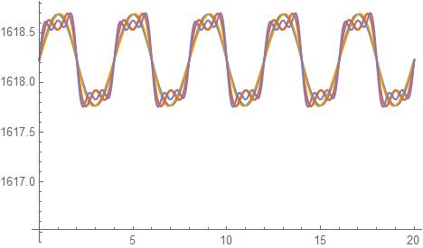
Plot[Evaluate[partialsums], {x, 0, 20}]

But the following is the result I see when I try to plot my partial sums and f together in a same range, for example, of 20.

Plot[{Evaluate[partialsums], f[x_]}, {x, 0, 20}]

In other words, Mathematica doesn't plot the partial sums together with my original function I want to compare it with.

I also tried with

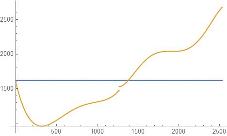
  Plot[{s[1, x], f[x_]}, {x, 0, 2530}]

But that doesn't work either. Moreover the function generated by the partial sums doesn't seem to follow the curvature of f and its amplitude.

I think I have probably made some mistakes in the calculus of the coefficients or in definition of variables, and until this is corrected, I can't go on with my analisys.

Could someone please help me?

Answer 1

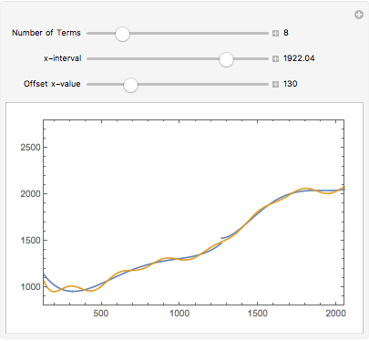
This is what I propose after correcting typos and errors. As the function in limited to an interval (band-limited), Fourier Analysis is valid considering that your function is periodic, with a period being the interval length. Thus, you can do this analysis. Otherwise, you should do Fourier Transform:

a0 = (2/2529)*(Integrate[f[x], {x, 0, 2529}]);
ak[n_?NumericQ] := (2/2529)*(NIntegrate[f[x]*Cos[2 \[Pi] n x/2529], {x, 0, 2529}]);
bk[n_?NumericQ] := (2/2529)*(NIntegrate[f[x]*Sin[2 \[Pi] n x/2529], {x, 0, 2529}]);
s[0, x_] := a0/2;
s[k_ /; k != 0, x_] := s[0, x] + 
Sum[ak[n]*Cos[2 \[Pi] n x/2529] + bk[n]*Sin[2 \[Pi] n x/2529], {n, 
 1, k}];
Manipulate[Plot[Evaluate@{f[x], s[n, x]}, {x, offset, offset + range}, 
PlotRange -> {offset, offset + range}, {800, 2800}}, Frame -> True, Axes -> False], 
{{n, 0, "Number of Terms"}, 0, 50, 1, Appearance -> "Labeled"}, 
{{range, 10, "x-interval"}, 0, 2529 - offset, Appearance -> "Labeled"}, 
{{offset, 0, "Offset x-value"}, 0, 2529 - range, 10, Appearance -> "Labeled"}, 
ContinuousAction -> False]

You can play with the number of terms, origin of analysis (x-axis origin), and range of x-values.

EDIT

A more compact code (assuming 50 terms for the sum):

Manipulate[Plot[Evaluate@{f[x], a0/2 + Sum[coeffs[[n]].(#[2 \[Pi] n x/2529] & /@ {Cos, Sin}), 
{n, 1, k}]}, {x, offset, offset + range}, 
PlotRange -> {{offset, offset + range}, {800, 2800}}, Frame -> True,
Axes -> False], 
{{k, 0, "Number of Terms"}, 0, 50, 1, Appearance -> "Labeled"}, 
{{range, 10, "x-interval"}, 0, 2529 - offset, 10, Appearance -> "Labeled"}, 
{{offset, 0, "Offset x-value"}, 0, 2529 - range, 10, Appearance -> "Labeled"}, 
ContinuousAction -> False, 
Initialization :> (coeffs = Table[(2/2529)*(NIntegrate[f[x]*(#[2 \[Pi] n x/2529] & /@ {Cos, Sin}), 
{x, 0,2529}]), {n, 1, 50}]; 
a0 = (2/2529)*(Integrate[f[x], {x, 0, 2529}]))]