added 776 characters in body
Source Link

EDIT

A more compact code (assuming 50 terms for the sum):

Manipulate[Plot[Evaluate@{f[x], a0/2 + Sum[coeffs[[n]].(#[2 \[Pi] n x/2529] & /@ {Cos, Sin}), 
{n, 1, k}]}, {x, offset, offset + range}, 
PlotRange -> {{offset, offset + range}, {800, 2800}}, Frame -> True,
Axes -> False], 
{{k, 0, "Number of Terms"}, 0, 50, 1, Appearance -> "Labeled"}, 
{{range, 10, "x-interval"}, 0, 2529 - offset, 10, Appearance -> "Labeled"}, 
{{offset, 0, "Offset x-value"}, 0, 2529 - range, 10, Appearance -> "Labeled"}, 
ContinuousAction -> False, 
Initialization :> (coeffs = Table[(2/2529)*(NIntegrate[f[x]*(#[2 \[Pi] n x/2529] & /@ {Cos, Sin}), 
{x, 0,2529}]), {n, 1, 50}]; 
a0 = (2/2529)*(Integrate[f[x], {x, 0, 2529}]))]
Source Link

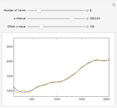
This is what I propose after correcting typos and errors. As the function in limited to an interval (band-limited), Fourier Analysis is valid considering that your function is periodic, with a period being the interval length. Thus, you can do this analysis. Otherwise, you should do Fourier Transform:

a0 = (2/2529)*(Integrate[f[x], {x, 0, 2529}]);
ak[n_?NumericQ] := (2/2529)*(NIntegrate[f[x]*Cos[2 \[Pi] n x/2529], {x, 0, 2529}]);
bk[n_?NumericQ] := (2/2529)*(NIntegrate[f[x]*Sin[2 \[Pi] n x/2529], {x, 0, 2529}]);
s[0, x_] := a0/2;
s[k_ /; k != 0, x_] := s[0, x] + 
Sum[ak[n]*Cos[2 \[Pi] n x/2529] + bk[n]*Sin[2 \[Pi] n x/2529], {n, 
 1, k}];
Manipulate[Plot[Evaluate@{f[x], s[n, x]}, {x, offset, offset + range}, 
PlotRange -> {offset, offset + range}, {800, 2800}}, Frame -> True, Axes -> False], 
{{n, 0, "Number of Terms"}, 0, 50, 1, Appearance -> "Labeled"}, 
{{range, 10, "x-interval"}, 0, 2529 - offset, Appearance -> "Labeled"}, 
{{offset, 0, "Offset x-value"}, 0, 2529 - range, 10, Appearance -> "Labeled"}, 
ContinuousAction -> False]

enter image description here

You can play with the number of terms, origin of analysis (x-axis origin), and range of x-values.