How to plot function over interval returned by Reduce[]

Question

Let $f(x) = (x^2 + 1) / x$. I need to plot the function for the values of $x$ in which the square of the function is larger than 4, and its cube is smaller than 64. So I used Reduce like this:

Reduce[((x^2 + 1)/x)^2 > 4 && ((x^2 + 1)/x)^3 < 64, x, Reals]

Now I am having problems plotting this. I need to use Plot to display the function on the specific interval, but I do not know how to input the result from Reduce (which may be union of intervals) in Plot in order to draw the function only for those values of $x$. Could anyone assist?

Answer 1

You can use your conditions directly with ConditionalExpression without going through Reduce:

  Plot[ConditionalExpression[(x^2 + 1)/ x,
    ((x^2 + 1)/x)^2 > 4 && ((x^2 + 1)/x)^3 < 64], {x, -3, 3}]

gives

Similarly, you get the same result using Piecewise:

 Plot[Piecewise[{{(x^2 + 1)/x,  ((x^2 + 1)/x)^2 > 4 && ((x^2 + 1)/x)^3 < 64}}, 
       Indeterminate], {x, -3, 3}]

If have to use Reduce, it can be used with ConditionalExpression and Piecewise as follows:

  Plot[Evaluate@ConditionalExpression[(x^2 + 1)/x, 
     Reduce[((x^2 + 1)/x)^2 > 4 && ((x^2 + 1)/x)^3 < 64, x, Reals]], {x, -3, 3}]
  Plot[Evaluate@Piecewise[{{(x^2 + 1)/x,
    Reduce[((x^2 + 1)/x)^2 > 4 && ((x^2 + 1)/x)^3 < 64, x, Reals]}},
     Indeterminate], {x, -3, 3}]

Both give the same output as above.

Answer 2

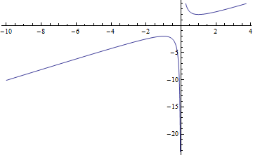
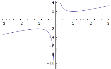
There are two subproblems: finding a reasonable plot range and restricting the graph to a subset of that range.

The following is somewhat brute force, but it is clear and general. It begins in the same way, by defining the function to plot (because it will be invoked several times):

f[x_] := (x^2 + 1)/x

We will also invoke the constraints twice, so let's put them into a function, too:

g[x_] := f[x]^2 > 4 && f[x]^3 < 64

(Reduce could be used here to speed up future calls to g, but it is not necessary. In other cases Reduce could fail to find a solution, so avoiding it provides a more general approach to plotting.)

We use numerical methods to find a finite plotting interval because there's no point to getting exact symbolic solutions for a plot. The idea is to maximize and minimize $x$ subject to the constraints, but limiting the search to an interval to make sure that finite endpoints are obtained:

xlim = x /. Last[#[{x, g[x], -10 <= x <= 10}, x]] & /@ {NMinimize, NMaximize}

Assemble this information into the plot:

Plot[If[g[x], f[x]], Evaluate @ {x, Sequence @@ xlim}]

In principle, the left limit of this plot should be $-\infty$; it was truncated at $-10$ by the interval constraints provided to NMaximize and NMinimize. Without that truncation the plot could not be created.