7
$\begingroup$

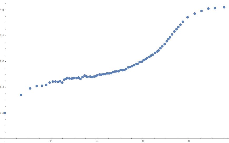
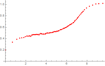
I'm researching data which looks somewhat like this:

data

I want to research it's properties, and for that I'd like to approximate it with a function.

Most of the data could be approximated with a x^3 + b x^2 + c x + d, except that the function that should be approximated by this should has a limit at somewhere around 1.05-1.1

So far, I've tried fitting the data to a + b CDF[NormalDistribution[c,d],x] + e CDF[NormalDistribution[g,h],x], since if a fit would be found that would work for me. However, matches that FindFit finds aren't even close to the data.

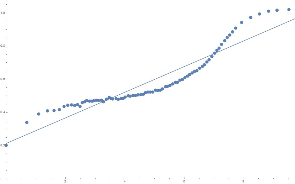
For example, here's default approximation:

    In[383]:= fit = 
 FindFit[aww, 
  a + b CDF[NormalDistribution[c, d], x] + 
   e CDF[NormalDistribution[f, g], x], {a, b, c, d, e, f, g}, x]

Out[383]= {a -> 8.63749, b -> 95.1976, c -> 385.463, d -> 663.707, 
 e -> -75.2157, f -> -85.3431, g -> -1038.96}

fitted function

Another thing I'm looking for is to use as few parameters (a,b,c,d,e,f,g) as possible in the approximation.

Should I try a different function, or is there a better way to find the fit?

Here's the data I'm working with:

{{0, 0.201519}, {0.693147, 0.339104}, {1.09861, 0.390401}, {1.38629, 
  0.410394}, {1.60944, 0.412307}, {1.79176, 0.417754}, {1.94591, 
  0.435408}, {2.07944, 0.444448}, {2.19722, 0.44524}, {2.30259, 
  0.442406}, {2.3979, 0.447151}, {2.48491, 0.437103}, {2.56495, 
  0.459182}, {2.63906, 0.46491}, {2.70805, 0.471748}, {2.8029, 
  0.468653}, {2.89037, 0.467473}, {2.94444, 0.469316}, {3.02013, 
  0.473278}, {3.11327, 0.47169}, {3.19846, 0.474257}, {3.27697, 
  0.464787}, {3.3669, 0.47889}, {3.46549, 0.49119}, {3.54085, 
  0.483291}, {3.58352, 0.481487}, {3.69704, 0.482514}, {3.77617, 
  0.479843}, {3.87106, 0.482569}, {3.94135, 0.485608}, {4.00722, 
  0.493137}, {4.1106, 0.5}, {4.17863, 0.498063}, {4.27102, 
  0.501595}, {4.35004, 0.501828}, {4.4347, 0.506954}, {4.5269, 
  0.508308}, {4.61155, 0.509924}, {4.68992, 0.518376}, {4.76985, 
  0.522628}, {4.84523, 0.523864}, {4.93102, 0.523511}, {5.02758, 
  0.533681}, {5.10417, 0.533301}, {5.18193, 0.5349}, {5.26333, 
  0.542174}, {5.36073, 0.555209}, {5.43189, 0.557592}, {5.51772, 
  0.563697}, {5.61202, 0.571544}, {5.70691, 0.582026}, {5.76335, 
  0.582014}, {5.85009, 0.5952}, {5.93492, 0.59866}, {6.01713, 
  0.610044}, {6.11193, 0.619297}, {6.17291, 0.628049}, {6.26708, 
  0.637543}, {6.34656, 0.64715}, {6.41987, 0.652515}, {6.51345, 
  0.666603}, {6.61286, 0.678222}, {6.67611, 0.686927}, {6.7542, 
  0.703593}, {6.83354, 0.718134}, {6.92997, 0.735695}, {7.0236, 
  0.757207}, {7.09035, 0.773825}, {7.16482, 0.788462}, {7.25558, 
  0.81023}, {7.36073, 0.833882}, {7.44522, 0.852115}, {7.52476, 
  0.867163}, {7.62487, 0.885581}, {7.72828, 0.909325}, {7.93179, 
  0.94279}, {8.23179, 0.97279}, {8.53179, 0.99279}, {8.83179, 
  1.01079}, {9.11788, 1.01579}, {9.11788, 1.01579}, {9.51788, 1.0209}}
$\endgroup$
7
  • 1
    $\begingroup$ Similar/duplicate: mathematica.stackexchange.com/questions/115444/… $\endgroup$
    – Michael E2
    Commented May 17, 2017 at 20:32
  • 1
    $\begingroup$ I'd recommend adding two additional pieces of information so that you can get more out of this: (1) How was the data generated? Is this set of measurements over time from a single instrument? (2) Is there a need to extrapolate outside the range of the data or do you just need to describe (rather than explain) the data within the observed range of predictor values? $\endgroup$
    – JimB
    Commented May 17, 2017 at 20:35
  • $\begingroup$ This is a processed data collected by a single instrument over several years, and indeed I want to extrapolate outside of the data range $\endgroup$ Commented May 17, 2017 at 20:37
  • 1
    $\begingroup$ Try MaxIterations -> 10000, Method -> NMinimize options of FindFit, it takes a minute but converges pretty nicely to {a -> 1.04317, b -> -0.528186, c -> 7.07308, d -> -1.14349, e -> -6.78146*10^6, f -> -46.0665, g -> -8.60979} $\endgroup$
    – swish
    Commented May 17, 2017 at 20:53
  • 1
    $\begingroup$ If you want to extrapolate past 10, you really ought to have some theoretically-based function as you have no predictor values larger than 9.5. The data alone can't do it for you. $\endgroup$
    – JimB
    Commented May 17, 2017 at 20:54

4 Answers 4

18
$\begingroup$

Extrapolation where you have no data and no theoretically-based curve is risky business (unless you're selling fake news where it seems to have the desired effect).

Update

If one smooths the data before fitting, that is a big no-no. It induces serial correlation (which the fitted model assumes doesn't exist), causes the estimates of precision (standard errors of parameters and confidence and prediction bands) to be much smaller than they should be, and gets you less precise estimates of the parameters. It's done all of the time and one of the things that has kept me in business all of these years. So the moral is: Don't do it!

End of Update

One can, however, obtain prediction intervals conditional on the chosen model. But, again, this does not address any uncertainty with the chosen model form especially if there is no theoretically based curve form.

So at minimum one should create confidence or prediction bands based on the chosen model. That can be done with NonlinearModelFit and the starting values and recommendations of @swish:

nlm = NonlinearModelFit[aww, a + b CDF[NormalDistribution[c, d], x] +
  e CDF[NormalDistribution[f, g], x],
  {{a, 1.0431}, {b, -0.5282}, {c, 7.0730}, {d, -1.1435}, {e, -5.3846*^6},
  {f, -45.37464}, {g, -8.5473}}, x, MaxIterations -> 100000];

A plot of the fit and 95% single prediction bands follows:

bands95[x_] = nlm["SinglePredictionBands"];
Show[Plot[{nlm[x], bands95[x]}, {x, Min[aww[[All, 1]]], 15}], ListPlot[aww]]

Prediction bands

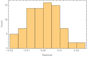
Further one should always look at the residuals. Here is the histogram of the residuals:

Histogram[nlm["FitResiduals"], Frame -> True, FrameLabel -> {"Residual", "Count"}]

Histogram of residuals

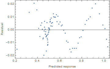
And a plot of the residuals vs the predicted values can suggest where there is a consistent lack of fit:

ListPlot[Transpose[{nlm["PredictedResponse"], nlm["FitResiduals"]}],
 Frame -> True, FrameLabel -> {"Predicted response", "Residual"}]

Residuals vs predicted

$\endgroup$
8
  • $\begingroup$ this is really cool! I'm gonna use this maaaany times in the future! $\endgroup$ Commented May 17, 2017 at 22:58
  • 2
    $\begingroup$ Upvoted for the first sentence. $\endgroup$ Commented May 18, 2017 at 7:15
  • $\begingroup$ I have another question about residuals. You are assuming that they are distributed normally. Does Mathematica have a function that can be used to confirm or deny this? $\endgroup$ Commented May 18, 2017 at 13:07
  • 1
    $\begingroup$ I made no such assumption. The Histogram and QuantilePlot (which I didn't include) are used to look for gross departures from normality (bimodality, skewness, heavy tails, etc.) but I wouldn't recommend to test for that. Why? The "significance" of the test depends not only on the kind and size of the departures but the sample size you could afford. Almost certainly, having a large sample size will find small but practically insignificant departures. I think the bigger issue here is the lack of independence among the residual errors as can be seen from the residual vs predicted plot. $\endgroup$
    – JimB
    Commented May 18, 2017 at 15:15
  • 4
    $\begingroup$ Smoothing before fitting is a big no-no. It induces serial correlation (which the fitted model assumes doesn't exist), causes the estimates of precision (standard errors of parameters and confidence and prediction bands) to be much smaller than they should be, and gets you less precise estimates of the parameters. It's done all of the time and one of the things that has kept me in business all of these years. So the moral is: Don't do it! $\endgroup$
    – JimB
    Commented May 19, 2017 at 12:36
2
$\begingroup$
data = {{0, 0.201519}, {0.693147, 0.339104}, {1.09861, 
    0.390401}, {1.38629, 0.410394}, {1.60944, 0.412307}, {1.79176, 
    0.417754}, {1.94591, 0.435408}, {2.07944, 0.444448}, {2.19722, 
    0.44524}, {2.30259, 0.442406}, {2.3979, 0.447151}, {2.48491, 
    0.437103}, {2.56495, 0.459182}, {2.63906, 0.46491}, {2.70805, 
    0.471748}, {2.8029, 0.468653}, {2.89037, 0.467473}, {2.94444, 
    0.469316}, {3.02013, 0.473278}, {3.11327, 0.47169}, {3.19846, 
    0.474257}, {3.27697, 0.464787}, {3.3669, 0.47889}, {3.46549, 
    0.49119}, {3.54085, 0.483291}, {3.58352, 0.481487}, {3.69704, 
    0.482514}, {3.77617, 0.479843}, {3.87106, 0.482569}, {3.94135, 
    0.485608}, {4.00722, 0.493137}, {4.1106, 0.5}, {4.17863, 
    0.498063}, {4.27102, 0.501595}, {4.35004, 0.501828}, {4.4347, 
    0.506954}, {4.5269, 0.508308}, {4.61155, 0.509924}, {4.68992, 
    0.518376}, {4.76985, 0.522628}, {4.84523, 0.523864}, {4.93102, 
    0.523511}, {5.02758, 0.533681}, {5.10417, 0.533301}, {5.18193, 
    0.5349}, {5.26333, 0.542174}, {5.36073, 0.555209}, {5.43189, 
    0.557592}, {5.51772, 0.563697}, {5.61202, 0.571544}, {5.70691, 
    0.582026}, {5.76335, 0.582014}, {5.85009, 0.5952}, {5.93492, 
    0.59866}, {6.01713, 0.610044}, {6.11193, 0.619297}, {6.17291, 
    0.628049}, {6.26708, 0.637543}, {6.34656, 0.64715}, {6.41987, 
    0.652515}, {6.51345, 0.666603}, {6.61286, 0.678222}, {6.67611, 
    0.686927}, {6.7542, 0.703593}, {6.83354, 0.718134}, {6.92997, 
    0.735695}, {7.0236, 0.757207}, {7.09035, 0.773825}, {7.16482, 
    0.788462}, {7.25558, 0.81023}, {7.36073, 0.833882}, {7.44522, 
    0.852115}, {7.52476, 0.867163}, {7.62487, 0.885581}, {7.72828, 
    0.909325}, {7.93179, 0.94279}, {8.23179, 0.97279}, {8.53179, 
    0.99279}, {8.83179, 1.01079}, {9.11788, 1.01579}, {9.11788, 
    1.01579}, {9.51788, 1.0209}};

{xmin, xmax} = MinMax[data[[All, 1]]];

order = 4;

coef = Array[a[# - 1] &, order + 1];

model = Piecewise[{
    {coef.xmax^Range[0, order], x > xmax},
    {coef.x^Range[0, order], xmin <= x <= xmax}}];

nlm = NonlinearModelFit[data, model, coef, x];

f[x_] = nlm // Normal

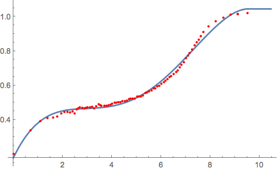
enter image description here

Plot[f[x], {x, xmin, 1.1 xmax},
 PlotStyle -> Thick,
 Epilog -> {Red , AbsolutePointSize[3], Point[data]}]

enter image description here

$\endgroup$
3
  • $\begingroup$ I'm making this model so I can research the behavior outside of the data bonds, and polynomials are generally not good for this. Power 4 polynomial will likely show some extreme values after, not approach a limit like I need it to $\endgroup$ Commented May 17, 2017 at 21:46
  • 1
    $\begingroup$ This is not a polynomial. It is zero below xmin ("I don't care how it behaves below 0") and hard limited at x > xmax ("upper range (10+) is important and it should approach some sort of limit"). $\endgroup$
    – Bob Hanlon
    Commented May 17, 2017 at 21:53
  • $\begingroup$ heh! better than any other alternatives I see so far $\endgroup$ Commented May 17, 2017 at 21:55
1
$\begingroup$

I copied your data and placed it in a variable called data.

ListPlot[data, PlotStyle -> Red]

Mathematica graphics

I made a slight change to the symbol names and used Erfc rather than CDF[NormalDistribution[...]]. Note that:

CDF[NormalDistribution[μ1, σ1], x]

can be written in the equivalent form

1/2 Erfc[(μ1 - x)/(Sqrt[2] σ1)]

So the model becomes:

model = a + 1/2 b1 Erfc[(μ1 - x)/(Sqrt[2] σ1)] + 
            1/2 b2 Erfc[(μ2 - x)/(Sqrt[2] σ2)]

I used NonlinearModelFit with the starting values shown below:

nlm = NonlinearModelFit[data, model,
   {
    {a, 1.0},
    {b1, -0.5}, {μ1, 7.0}, {σ1, -1.1},
    {b2, -50}, {μ2, -10}, {σ2, -4}
    },
   x,
   MaxIterations -> 100000
   ];

It gave a warning message about convergence but produced an answer:

nlm["BestFitParameters"]
(* {a -> 1.04319, 
 b1 -> -0.526302, μ1 -> 7.07431, σ1 -> -1.14011, 
 b2 -> -1.94269*10^213, μ2 -> -1507.49, σ2 -> -48.2558} *)

Note the huge bizarre negative value for b2 and the very large negative values for the mean and standard deviation.

Here is the correlation matrix

Mathematica graphics

This states that the latter three parameters have no resolution. Change two of them and the third will follow.

Rather than being a 7 parameter problem we really have only 5 parameters. I set b2 and μ1 to arbitrary values of -50 and -10 and allowed the optimizer to pick the standard deviation.

nlmFixed = NonlinearModelFit[data,
   a + 1/2 b1 Erfc[(μ1 - x)/(Sqrt[2] σ1)] - 
    50/2  Erfc[(-10 - x)/(Sqrt[2] σ2)],
   {
    {a, 1.0},
    {b1, -0.5}, {μ1, 7.0}, {σ1, -1.0},
    {σ2, -4}
    },
   x,
   MaxIterations -> 100000
   ];

nlmFixed["BestFitParameters"]

(* {a -> 1.04815, 
 b1 -> -0.546963, μ1 -> 7.05788,
 σ1 -> -1.20422, σ2 -> -3.96872} *)

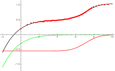
Now a plot shows the results (I included the two Erfc components).

Show[
 Plot[Evaluate[{
     a + 1/2 b1 Erfc[(μ1 - x)/(Sqrt[2] σ1)]
         - 50/2 Erfc[(-10 - x)/(Sqrt[2] σ2)], 
         1/2 b1 Erfc[(μ1 - x)/(Sqrt[2] σ1)],
        - 50/2  Erfc[(-10 - x)/(Sqrt[2] σ2)]
     } /. nlmFixed["BestFitParameters"]], 
  {x, -2, 10},
   PlotStyle -> {Black, Red, Green},
  PlotLegends -> {"Model", "Erfc 1", "Erfc2"}
  ],
 ListPlot[data, PlotStyle -> Red],
 PlotRange -> {Automatic, All},
 ImageSize -> 450
 ]

Mathematica graphics

$\endgroup$
1
$\begingroup$

For fun, I decided to explore this data set a bit to see if I could find something that fits nicely.

I began with the following expression:

 model=a +b (c -d* 2.718281828459045`^(1/(2.` +2.718281828459045`^x x)-1.` E^(e* x^4)))^2 

I then used Mathematica's NonLinearModelFit function to find the values for a, b, c, d, and e.

nlm = NonlinearModelFit[Transpose@data, model, {a, b, c, d, e}, x];

nlm["BestFitParameters"]

Out[301]= {a -> 0.114274, b -> 0.947472, c -> 0.983351, d -> 1.03142, e -> 0.000259904}

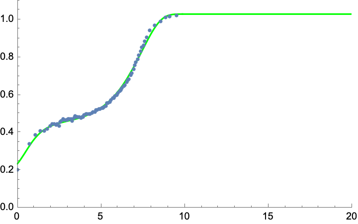
This gives a fit that looks like:

enter image description here

It was mentioned in the original post that we expect a limit of around 1.05-1.1, which appears to be captured by this model.

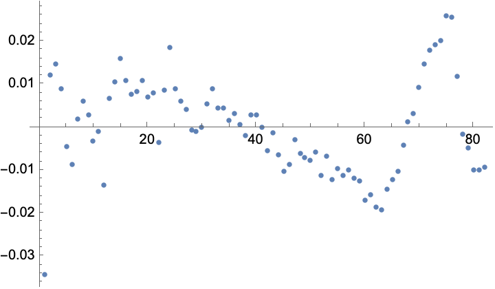
Plotting the residuals we see the following:

enter image description here

Enjoy!

$\endgroup$

Your Answer

By clicking “Post Your Answer”, you agree to our terms of service and acknowledge you have read our privacy policy.

Not the answer you're looking for? Browse other questions tagged or ask your own question.