Added sermon about smoothing prior to fitting as the OP has confessed to doing so.
Source Link
JimB
  • 42.9k
  • 3
  • 51
  • 108

Extrapolation where you have no data and no theoretically-based curve is risky business (unless you're selling fake news where it seems to have the desired effect).

Update

If one smooths the data before fitting, that is a big no-no. It induces serial correlation (which the fitted model assumes doesn't exist), causes the estimates of precision (standard errors of parameters and confidence and prediction bands) to be much smaller than they should be, and gets you less precise estimates of the parameters. It's done all of the time and one of the things that has kept me in business all of these years. So the moral is: Don't do it!

End of Update

One can, however, obtain prediction intervals conditional on the chosen model. But, again, this does not address any uncertainty with the chosen model form especially if there is no theoretically based curve form.

So at minimum one should create confidence or prediction bands based on the chosen model. That can be done with NonlinearModelFit and the starting values and recommendations of @swish:

nlm = NonlinearModelFit[aww, a + b CDF[NormalDistribution[c, d], x] +
  e CDF[NormalDistribution[f, g], x],
  {{a, 1.0431}, {b, -0.5282}, {c, 7.0730}, {d, -1.1435}, {e, -5.3846*^6},
  {f, -45.37464}, {g, -8.5473}}, x, MaxIterations -> 100000];

A plot of the fit and 95% single prediction bands follows:

bands95[x_] = nlm["SinglePredictionBands"];
Show[Plot[{nlm[x], bands95[x]}, {x, Min[aww[[All, 1]]], 15}], ListPlot[aww]]

Prediction bands

Further one should always look at the residuals. Here is the histogram of the residuals:

Histogram[nlm["FitResiduals"], Frame -> True, FrameLabel -> {"Residual", "Count"}]

Histogram of residuals

And a plot of the residuals vs the predicted values can suggest where there is a consistent lack of fit:

ListPlot[Transpose[{nlm["PredictedResponse"], nlm["FitResiduals"]}],
 Frame -> True, FrameLabel -> {"Predicted response", "Residual"}]

Residuals vs predicted

Extrapolation where you have no data and no theoretically-based curve is risky business (unless you're selling fake news where it seems to have the desired effect).

One can, however, obtain prediction intervals conditional on the chosen model. But, again, this does not address any uncertainty with the chosen model form especially if there is no theoretically based curve form.

So at minimum one should create confidence or prediction bands based on the chosen model. That can be done with NonlinearModelFit and the starting values and recommendations of @swish:

nlm = NonlinearModelFit[aww, a + b CDF[NormalDistribution[c, d], x] +
  e CDF[NormalDistribution[f, g], x],
  {{a, 1.0431}, {b, -0.5282}, {c, 7.0730}, {d, -1.1435}, {e, -5.3846*^6},
  {f, -45.37464}, {g, -8.5473}}, x, MaxIterations -> 100000];

A plot of the fit and 95% single prediction bands follows:

bands95[x_] = nlm["SinglePredictionBands"];
Show[Plot[{nlm[x], bands95[x]}, {x, Min[aww[[All, 1]]], 15}], ListPlot[aww]]

Prediction bands

Further one should always look at the residuals. Here is the histogram of the residuals:

Histogram[nlm["FitResiduals"], Frame -> True, FrameLabel -> {"Residual", "Count"}]

Histogram of residuals

And a plot of the residuals vs the predicted values can suggest where there is a consistent lack of fit:

ListPlot[Transpose[{nlm["PredictedResponse"], nlm["FitResiduals"]}],
 Frame -> True, FrameLabel -> {"Predicted response", "Residual"}]

Residuals vs predicted

Extrapolation where you have no data and no theoretically-based curve is risky business (unless you're selling fake news where it seems to have the desired effect).

Update

If one smooths the data before fitting, that is a big no-no. It induces serial correlation (which the fitted model assumes doesn't exist), causes the estimates of precision (standard errors of parameters and confidence and prediction bands) to be much smaller than they should be, and gets you less precise estimates of the parameters. It's done all of the time and one of the things that has kept me in business all of these years. So the moral is: Don't do it!

End of Update

One can, however, obtain prediction intervals conditional on the chosen model. But, again, this does not address any uncertainty with the chosen model form especially if there is no theoretically based curve form.

So at minimum one should create confidence or prediction bands based on the chosen model. That can be done with NonlinearModelFit and the starting values and recommendations of @swish:

nlm = NonlinearModelFit[aww, a + b CDF[NormalDistribution[c, d], x] +
  e CDF[NormalDistribution[f, g], x],
  {{a, 1.0431}, {b, -0.5282}, {c, 7.0730}, {d, -1.1435}, {e, -5.3846*^6},
  {f, -45.37464}, {g, -8.5473}}, x, MaxIterations -> 100000];

A plot of the fit and 95% single prediction bands follows:

bands95[x_] = nlm["SinglePredictionBands"];
Show[Plot[{nlm[x], bands95[x]}, {x, Min[aww[[All, 1]]], 15}], ListPlot[aww]]

Prediction bands

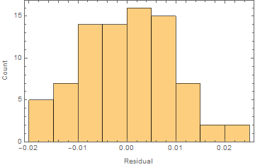
Further one should always look at the residuals. Here is the histogram of the residuals:

Histogram[nlm["FitResiduals"], Frame -> True, FrameLabel -> {"Residual", "Count"}]

Histogram of residuals

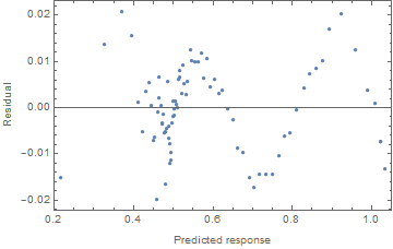
And a plot of the residuals vs the predicted values can suggest where there is a consistent lack of fit:

ListPlot[Transpose[{nlm["PredictedResponse"], nlm["FitResiduals"]}],
 Frame -> True, FrameLabel -> {"Predicted response", "Residual"}]
Residuals vs predicted

Source Link
JimB
  • 42.9k
  • 3
  • 51
  • 108

Extrapolation where you have no data and no theoretically-based curve is risky business (unless you're selling fake news where it seems to have the desired effect).

One can, however, obtain prediction intervals conditional on the chosen model. But, again, this does not address any uncertainty with the chosen model form especially if there is no theoretically based curve form.

So at minimum one should create confidence or prediction bands based on the chosen model. That can be done with NonlinearModelFit and the starting values and recommendations of @swish:

nlm = NonlinearModelFit[aww, a + b CDF[NormalDistribution[c, d], x] +
  e CDF[NormalDistribution[f, g], x],
  {{a, 1.0431}, {b, -0.5282}, {c, 7.0730}, {d, -1.1435}, {e, -5.3846*^6},
  {f, -45.37464}, {g, -8.5473}}, x, MaxIterations -> 100000];

A plot of the fit and 95% single prediction bands follows:

bands95[x_] = nlm["SinglePredictionBands"];
Show[Plot[{nlm[x], bands95[x]}, {x, Min[aww[[All, 1]]], 15}], ListPlot[aww]]

Prediction bands

Further one should always look at the residuals. Here is the histogram of the residuals:

Histogram[nlm["FitResiduals"], Frame -> True, FrameLabel -> {"Residual", "Count"}]

Histogram of residuals

And a plot of the residuals vs the predicted values can suggest where there is a consistent lack of fit:

ListPlot[Transpose[{nlm["PredictedResponse"], nlm["FitResiduals"]}],
 Frame -> True, FrameLabel -> {"Predicted response", "Residual"}]
Residuals vs predicted