1
$\begingroup$

I have some data in a .txt file, and I'm trying to import it to Mathematica and fit it with a function. The data is a 647x647 matrix of values. This seems like it should work:

data = Import["C:\\File_path_goes_here.txt", "Table"];
curve = NonlinearModelFit[data, a*Sin[c*x + d*y + e] + b, {a, b, c, d, e}, {x,y}]

But I get the message

Number of coordinates (647) is not equal to the number of variables (2).

I know the data import works, because I can plot the data with ArrayPlot[data], so it must be something with the way I'm trying to do the fit. Is the "Table" format incompatible with the NonlinearModelFit function? If so, how do I convert it to a compatible format, or alternatively, what function should I use to fit that model with that dataset? If not, is my syntax wrong in some way? Thank you for the help!

$\endgroup$
2
  • 1
    $\begingroup$ The problem is: You have two independent variables x,y and mathematica wants to insert the values of the data-matrix into those values to fit the parameters a,b,c,d,e,f, but your matrix is 647x647. So the question for me (and therefore also for mathematica) is: How to gather value-pairs to use for (x,y)? I would have expected a matrix with N rows and 2 columns, then it would be clear (like in the first example here: reference.wolfram.com/language/ref/NonlinearModelFit.html) $\endgroup$
    – tim
    Commented Jan 7, 2015 at 10:54
  • $\begingroup$ So the data is a scan of the height of some surface. The rows and columns of the matrix correspond to different positions on the surface, and the value at that position of the matrix corresponds to the height at that point. It's a square scan, 647 pixels in each direction. Does that help clarify? $\endgroup$ Commented Jan 7, 2015 at 12:54

1 Answer 1

3
$\begingroup$

First, let's create some data:

dataZ = Table[RandomReal[{0.9, 1.1}]*Sin[x + y] + RandomReal[{-.1, .1}], 
              {x, 0, 2, .1},
              {y, 0, 2, .1}];

Now we can use MapIndexed in order to add the missing x and y values:

dataYXZ = Flatten[MapIndexed[Append[2 (#2 - 1)/20, #1] &, dataZ, {2}], 1];

Notice that MapIndexed positions need to be adjusted to match the original x and y ranges. Then we can do the curve fitting:

curve = NonlinearModelFit[dataYXZ, a*Sin[c*x + d*y + e] + b, {a, b, c, d, e}, {x, y}]

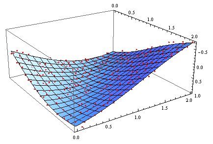
And verify with a plot

Show[Plot3D[Evaluate@curve[x, y], {x, 0, 2}, {y, 0, 2}], 
     Graphics3D[{Red, Point@dataYXZ}]]

enter image description here

$\endgroup$
4
  • 1
    $\begingroup$ Ah, awesome - I think this is exactly what I needed!! Thank you so much! One last question - if the data is asymmetric, ie 500 in one direction and 1000 in another direction, what would I need to change in this basic approach? $\endgroup$ Commented Jan 7, 2015 at 13:31
  • $\begingroup$ In that case you will have to change the 2 (#2 - 1)/20 with something more complex. The "Rescale" command will help you with this. $\endgroup$ Commented Jan 7, 2015 at 13:54
  • $\begingroup$ Great, I'll dig into it and figure it out. Thank you so much again! $\endgroup$ Commented Jan 7, 2015 at 14:05
  • 1
    $\begingroup$ Just commenting again now that I'm done - I found that for an asymmetric dataset, it was actually easier to use: Flatten[MapIndexed[Append[#2, #1] &, data, {2}], 1] And then just readjust my indexes after the fact. $\endgroup$ Commented Jan 7, 2015 at 15:00

Your Answer

By clicking “Post Your Answer”, you agree to our terms of service and acknowledge you have read our privacy policy.

Not the answer you're looking for? Browse other questions tagged or ask your own question.