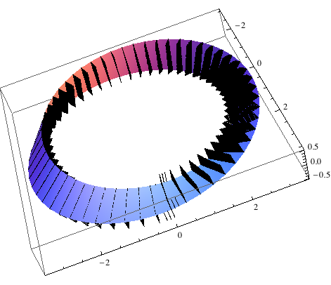
The question is pretty much in the title; I'm about to teach my multivariable calculus students about orientations on surfaces, and I would like to be able to show them pictures. Any ideas?
4 Answers
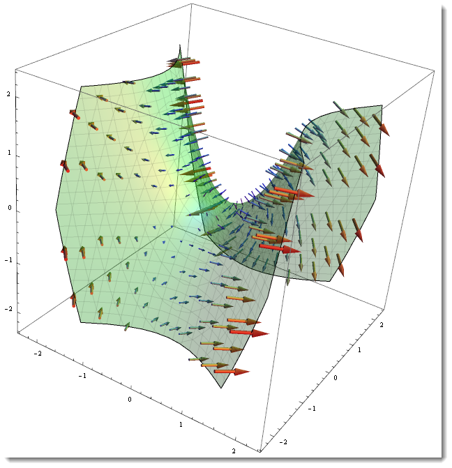
The easiest thing to do is differentiate the field and use VectorPlot3D and ContourPlot3D to show orthogonality of these. This is from Documentation Center. I will change this a bit from original to polish graphics for your lecture. These are not unit vectors though - do u really need unit ones? It can be done too if you need.
Use a contour plot to visualize the region of a vector plot:
scalarField = x^2 - y^2 - z;
vectorField = D[scalarField, {{x, y, z}}]
Plot a vector field over a particular region:
v = VectorPlot3D[vectorField, {x, -2, 2}, {y, -2, 2}, {z, -2, 2},
  VectorPoints -> 20, VectorScale -> {0.1, Scaled[0.5]},
  RegionFunction -> Function[{x, y, z}, -0.1 <= scalarField <= 0.1],
  VectorStyle -> "Arrow3D", VectorColorFunction -> "Rainbow"]
Create a contour plot of the vector plot's region:
c = ContourPlot3D[
  scalarField == 0, {x, -2, 2}, {y, -2, 2}, {z, -2, 2}, Mesh -> 20,
  MeshStyle -> Opacity[.1],
  ContourStyle -> Directive[Green, Opacity[0.3], Specularity[White, 30]]]
Combine the vector and contour plots:
Show[v, c]
-
$\begingroup$ This is very helpful, thanks! Is there any way to modify your idea so that it works for surfaces described by parametric equations, rather than as level surfaces of functions of $x$, $y$, and $z$? $\endgroup$ Commented Nov 6, 2012 at 21:39
-
$\begingroup$ @PaulSiegel I modified my answer to show a way to get vector field for surfaces on parametric form. $\endgroup$– sschCommented Nov 7, 2012 at 0:25
-
1$\begingroup$ Nice start--but this is not a unit normal field. The lengths of the arrows come from extraneous, irrelevant information related to the function of which this surface is a zero. (The fix is fairly easy to make--but watch out for places where the gradient is zero!) $\endgroup$– whuberCommented Nov 7, 2012 at 17:00
-
$\begingroup$ @whuber yes, I explicitly mentioned it in 1st paragraph. $\endgroup$ Commented Nov 7, 2012 at 17:02
-
2$\begingroup$ Sorry; I focused on the image and only skimmed the text! (+1). However, as I pointed out, the lengths of your vectors are extraneous to the problem, so in the intended application it likely is best to normalize them. You are also going to run into trouble where the gradient is zero (at the origin in your example) because you won't be able to calculate a nontrivial normal vector, even though it exists. $\endgroup$– whuberCommented Nov 8, 2012 at 16:33
Let's start with a parametrized surface. Any one will do, but I guess being orientable helps in this case.
Then calculate the unit normal, and then create a Manipulate object that lets you see how the normal behaves:
σ[u_, v_] := {(2 + Cos[v]) Cos[u], (2 + Cos[v]) Sin[u], Sin[v]}
n[u_, v_] := Evaluate[Normalize[
   Cross[D[σ[u, v], u], D[σ[u, v], v]]
   ]]
surfacePlot =
  ParametricPlot3D[σ[u, v], {u, -Pi, Pi}, {v, -Pi, Pi},
   PlotRangePadding -> 1];
normalPlot =
  ParametricPlot3D[n[u, v], {u, -Pi, Pi}, {v, -Pi, Pi},
   PlotStyle -> Opacity[0.5]];

Manipulate[
 {Show[{
    surfacePlot,
    Graphics3D[{Thick, Red,
      Arrow[{σ @@ pt, σ @@ pt + n @@ pt}]}]
    }],
  Show[{
    normalPlot,
    Graphics3D[{Thick, Red, Arrow[{{0, 0, 0}, n @@ pt}]}]
    }]
  }
 ,
 {pt, {-Pi, -Pi}, {Pi, Pi}}]
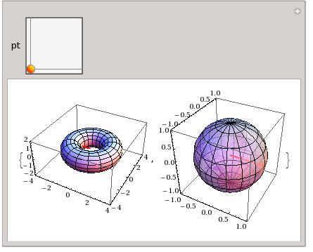
To show the entire vector field for a surface on parametric form you can use a bunch of Arrow's:
Show[{
  surfacePlot,
  Graphics3D[
   Table[
    Arrow[{σ[u, v], σ[u, v] + n[u, v]}],
    {u, -Pi, Pi, 0.4}, {v, -Pi, Pi, 0.4}]
   ]
  }]
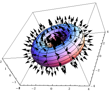
As you can see, the arrows are equally spaced in the parameter space, which leads to uneven distribution of arrows on the surface; it might be worth transforming the parametrization into $f(x,y,z)=0$ form to get a nicer result.
It isn't too hard to roll your own routine, of course:
UnitNormalVector[f_, {u_, u0_}, {v_, v0_}] := Block[{f0, g0},
                 f0 = f /. {u -> u0, v -> v0};
                 g0 = Transpose[D[f, {{u, v}}] /. {u -> u0, v -> v0}];
                 Arrow[{f0, f0 + Normalize[Cross @@ g0]}]]

(* Möbius strip *)
mobius[u_, v_] :=
      {(3 + (1/2 - v) Cos[u/2]) Cos[u], (3 + (1/2 - v) Cos[u/2]) Sin[u], (1/2 - v) Sin[u/2]}

Show[ParametricPlot3D[mobius[u, v], {u, 0, 2 π}, {v, 0, 1},
                      Mesh -> False, PlotPoints -> 55],
     Graphics3D[Table[UnitNormalVector[mobius[u, v], {u, u0}, {v, v0}],
                      {u0, 0, 2 π, 2 π/20}, {v0, 0, 1, 1/5}]], PlotRange -> All]
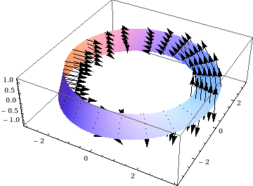
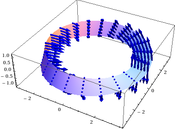
It's not too hard to give the arrows depicting the normals some style:
% /. Arrow[stuff__] :> {Blue, Arrow[Tube[stuff, 0.05]]}
-
3$\begingroup$ Orienting a Möbius strip is pure heresy. Voting to inquisite. $\endgroup$ Commented Nov 7, 2012 at 2:37
-
1$\begingroup$ @bel, you weren't aware that I've always had a heretical streak? >:) $\endgroup$ Commented Nov 7, 2012 at 2:44
-
-
1
Just adding this answer for completion seeing as there is an out-of-the-box solution for this hidden in the documentation.
Essentially the following function:
normalsShow[g_Graphics3D] :=
  Module[{pl, vl, n},
   {pl, vl} = First @ Cases[g,
      GraphicsComplex[pl_, prims_, VertexNormals -> vl_,
        opts___?OptionQ] :> {pl, vl}, ∞];
   n = Length[pl];
   Show[g,
    Graphics3D[
     GraphicsComplex @@ {Join[pl, pl + vl/3], {Black,
        Line[Table[{i, i + n}, {i, n}]]}}]]
   ];
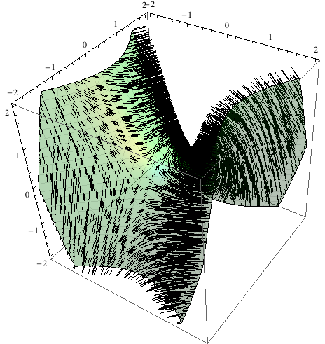
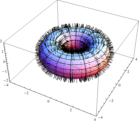
(that can easily be tweaked to subsample or use arrows instead of lines) works in the previously mentioned examples:
The c of Vitaly:
c // normalsShow
the donut:
surfacePlot // normalsShow
and the Möbius band:
ParametricPlot3D[mobius[u, v], {u, 0, 2 π}, {v, 0, 1},
  Mesh -> False, PlotPoints -> 55] // normalsShow
