Visibility Polygon

Question

Description

Based on recent assignment at work, I have become interested in computational geometry. So, I am trying to implement a visibility polygon as to explore some fundamental concepts and ideas.

The objective is to derive a visibility polygon. I have implemented a mock-up module, but I struggle to get the actual polygon... I was wondering if somebody could throw in some pointers on how to proceed.

Code:

Module[
 {module, vision, obstacle, bVision, bObstacle},
 module = Polygon[{{0, 0}, {10, 0}, {10, 8}, {5, 8}, {5, 12}, {0, 12}}];
 vision = Disk[{1, 1}, 5, {Pi/6, Pi/2}];
 obstacle = Rectangle[{2, 1}, {6, 3}, RoundingRadius -> .5];

 bVision = MeshCoordinates @ BoundaryDiscretizeRegion @ RegionDifference[vision, obstacle];
 bObstacle = MeshCoordinates @ BoundaryDiscretizeRegion @ obstacle;

 Graphics[{
   {FaceForm @ White, EdgeForm @ {Black, Thick}, module},
   {FaceForm @ White, EdgeForm @ {Black, Thick}, vision},
   {FaceForm @ White, EdgeForm @ {Blue, Thick}, obstacle},

   {Red, PointSize -> 0.015, Point @ bVision},
   {Green, PointSize -> 0.015, Point @ bObstacle},

   (*The idea was to use these lines for RegionIntersection...The idea failed...*)
   Line @ {{1, 1}, #} & /@ bVision

   }, ImageSize -> {300, 300}]
 ]

Reference

Visibility Polygon

Answer 1

Edit

• Test non-convex case.

Clear["Global`*"];
space0 = Rectangle[{0, 0}, {10, 12}];
obstacles0 = {Rectangle[{2, 1}, {6, 3}], 
   Annulus[{5, 5}, {1/2, 1}, {.2 Pi, 1.5 Pi}], 
   WindingPolygon[{7, 5} + # & /@ {{0.35, 0.2}, {0.9, 0.75}, {0.1, 
       0.55}, {0.9, 0.35}, {0.42, 0.9}}], Rectangle[{5, 8}, {10, 12}],
    Annulus[{3, 7}, {1/2, 1}, {Pi, 1.5 Pi}]};
domain = Fold[RegionDifference, BoundaryDiscretizeRegion@space0, 
   BoundaryDiscretizeRegion /@ obstacles0];
lines = MeshPrimitives[domain, 1][[;; , 1]];
L = 15;
shadow[loc_, line_] := 
  Polygon[{line[[1]] + L*Normalize[line[[1]] - loc], line[[1]], 
    line[[2]], line[[2]] + L*Normalize[line[[2]] - loc]}];
Manipulate[
 Graphics[{Orange, space0, AbsolutePointSize[10], Red, Point@loc, 
   Black, shadow[loc, #] & /@ lines, White, obstacles0}, 
  PlotRange -> RegionBounds[domain]], {{loc, {8, 1}}, Locator, 
  TrackingFunction -> Function[pos, loc = RegionNearest[domain]@pos], 
  Appearance -> 
   Graphics[{Red, AbsolutePointSize[10], Point[{0, 0}]}]}]

Original

• Now support dynamic.
• Only work for convex obstacles. For non-convex obstacles and non-convex space,we need to subdivide to several convex pieces at first.

Clear["Global`*"];
space0 = Rectangle[{0, 0}, {10, 12}];
obstacles0 = {Rectangle[{2, 1}, {6, 3}], Disk[{5, 5}, 1], 
   Polygon[{{7, 5}, {9, 5}, {8, 7}}], Rectangle[{5, 8}, {10, 12}]};
domain = BoundaryDiscretizeRegion@
   RegionDifference[space0, RegionUnion@obstacles0];
shadow[loc_, obstacle_] := 
  Module[{con, pts}, 
   con = ConvexHullMesh[
     Join[{loc}, MeshCoordinates[BoundaryDiscretizeRegion@obstacle]]];
   pts = MeshPrimitives[con, 1][[;; , 1]][[;; , 1]];
   RegionUnion[
    Polygon[{pts[[-1]], pts[[2]], 
      pts[[2]] + 100 (pts[[2]] - pts[[1]]), 
      pts[[01]] + 100 (pts[[-1]] - pts[[1]])}], obstacle]];
Manipulate[
 Graphics[{Orange, space0, AbsolutePointSize[10], Red, Point@loc, 
   Black, BoundaryDiscretizeRegion@
      RegionIntersection[space0, shadow[loc, #]] & /@ obstacles0, 
   White, obstacles0}], {{loc, {8, 1}}, Locator, 
  TrackingFunction -> Function[pos, loc = RegionNearest[domain]@pos], 
  Appearance -> Graphics[{Red, AbsolutePointSize[10], Point[{0, 0}]}]}]

Answer 2

The link provided by corey979 in the comments to the question does certainly look close to the desired outcome. However I'm not sure it would generalise (easily) to the case with objects within a bounding region also occluding the vision. Here is a method using RegionIntersection, it is relatively slow (around a second in my test cases), and ideally would have a recursive procedure added to refine the visibility polygon where needed.

Setup

space = Polygon[{{0, 0}, {10, 0}, {10, 8}, {5, 8}, {5, 12}, {0, 12}}];
obstacles = {Rectangle[{2, 1}, {6, 3}], Disk[{5, 5}, 1], Polygon[{{7, 5}, {9, 5}, {8, 7}}]};
reg = RegionDifference[DiscretizeGraphics[space], DiscretizeGraphics[obstacles, MaxCellMeasure -> 0.03]];

vision = CirclePoints[2., 200];(*Could be altered to only permit a viewing angle < 360*)

loc = {2, 5.5};

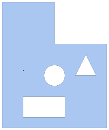
Show[reg, Graphics[Point[loc]]]

Solve

mp = MeshPrimitives[RegionBoundary[reg], 1];

polypts = Flatten[
    ParallelTable[
     Nearest[
      DeleteCases[
        RegionIntersection[#, HalfLine[{loc, loc + v}]] & /@ mp, 
        EmptyRegion[2]][[;; , 1]], 
     loc, 1],
    {v, vision}],
   1
  ];

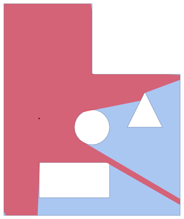
Show[reg, Graphics[{Point[loc], Opacity[0.5], Red, Polygon[polypts]}]]

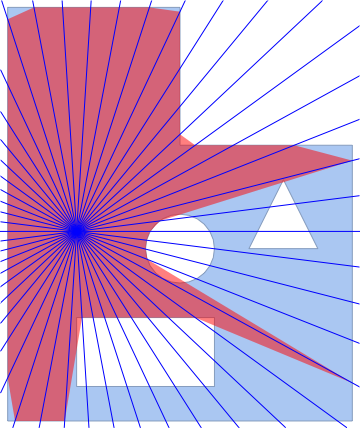
You can see that at the edges of occluding objects the vision polygon sometimes clips through them. This will be an artefact of this method that will reduce as the number of vision lines increases, however this slows the process down. Better would be to use a few vision lines at the outset (20, maybe 50?) and then recursively refine (by adding further vision lines) those regions where the distance from loc to the termination points of subsequent vision lines changes abruptly.

Here is an exaggerated illustration of the problem with the vision lines used shown in blue:

Answer 3

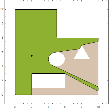
I am using v12.2.0 on Win7-x64. This is too slow for dynamic work but hopefully will be useful in more static cases, or at least as a verification aid while developing your own algorithms.

Clear["Global`*"];
space = Polygon[{{0, 0}, {10, 0}, {10, 8}, {5, 8}, {5, 12}, {0, 12}}];
obstacles = {Rectangle[{2, 1}, {6, 3}], Disk[{5, 5}, 1], 
   Polygon[{{7, 5}, {9, 5}, {8, 7}}]};
reg = RegionDifference[DiscretizeGraphics[space], 
   DiscretizeGraphics[obstacles, MaxCellMeasure -> 0.03]];
loc = {2, 5.5};

reg2 = Line[{loc, {x, y}}];
cond = RegionWithin[reg, reg2];

RegionPlot[cond
 , {x, -1, 11}, {y, -1, 13}
 , MaxRecursion -> 2
 , PlotPoints -> 30
 , PlotStyle -> ColorData[97][3]
 , BoundaryStyle -> Directive[Thin, Black]
 , Prolog -> {
   {Opacity[0.4, Brown], reg}
   }
 , Epilog -> {
   {Black, AbsolutePointSize[6]
    , Point@loc}
   }
 ]