0
$\begingroup$

I am studying the Landau Free Energy Equation. First of all the plot displayed only shown negative range. can i show the positive range too? (y-axes). Then, can I turn this plot into 2-D Plot?

α= 1;
β= 1;
Tmp = 0.1316;
ρ= 0.01;
T = -2;

FreeEnergy = 
  1/2*(T - 1)*P^2 + 1/4*P^4 + (1/2*α^2*β*M^2*(T - Tmp)) + 
  1/4 α^2*(β)*(M^4) + 1/2*(ρ*(P^2)*(M^2))

Plot3D[FreeEnergy, {M, -2.05216, 2.05217}, {P, -2.35669, 2.35669}]

enter image description here

Update

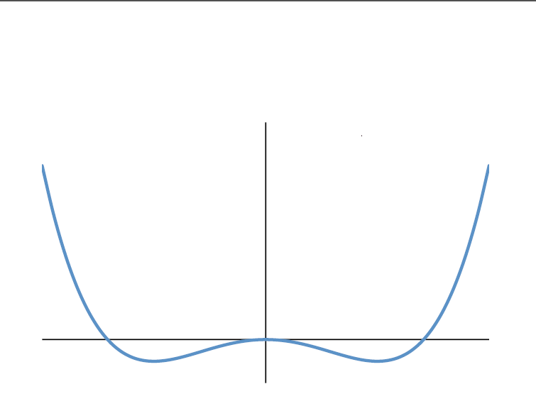
This what I want. It should be extended to the positive side. Maybe I should minimize the equation first?

enter image description here

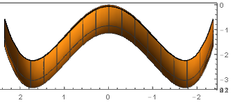
After use ViewPoint-> {-Infinity,0,0} i get this but still not quite right (because the orange part is showing and both left and right should extend to positive side like above picture).

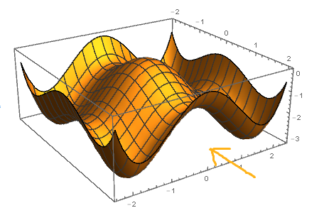
enter image description here

$\endgroup$
8
  • 1
    $\begingroup$ What do you mean by turning it into a 2D plot? Do you want a slice through it? A projection? A density plot? A contour plot? Also, your function doesn't take any positive values in the domain you've passed to Plot3D. You can set the displayed range manually with PlotRange though. $\endgroup$ Commented Apr 8, 2016 at 9:47
  • 2
    $\begingroup$ ContourPlot[FreeEnergy, {M, -2.05216, 2.05217}, {P, -2.35669, 2.35669}] and DensityPlot[FreeEnergy, {M, -2.05216, 2.05217}, {P, -2.35669, 2.35669}] are two examples of 2D plots of the 3D data $\endgroup$
    – Jason B.
    Commented Apr 8, 2016 at 9:48
  • 1
    $\begingroup$ @Nabil Something like using the ViewPoint -> {-Infinity, 0, 0} option? $\endgroup$ Commented Apr 8, 2016 at 10:03
  • 2
    $\begingroup$ Either Plot[Evaluate[FreeEnergy /. M -> 0], {P, -2.35669, 2.35669}] or Plot[Evaluate[FreeEnergy /. P -> 0], {M, -2.05216, 2.05217}]. $\endgroup$
    – m_goldberg
    Commented Apr 9, 2016 at 1:13
  • 2
    $\begingroup$ The reason you're not seeing any positive values in the graph is because the function doesn't take any positive values for the range you're plotting. Any reason you're not doing something like Plot3D[FreeEnergy, {M, -3, 3}, {P, -3, 3}] instead? $\endgroup$
    – user484
    Commented Apr 9, 2016 at 2:54

3 Answers 3

3
$\begingroup$

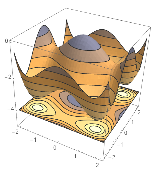
Assuming this is not just ContourPlot. Just minor changes:

α = 1;
β = 1;
tmp = 0.1316;
ρ = 0.01;
t = -2;

fe[m_, p_] := 
 1/2*(t - 1)*p^2 + 1/4*p^4 + (1/2*α^2*β*m^2*(t - tmp)) + 
  1/4 α^2*(β)*(m^4) + 1/2*(ρ*(p^2)*(m^2))

Now,

Show[SliceContourPlot3D[
  z - fe[m, p], {z == -4}, {m, -2.05216, 2.05217}, {p, -2.35669, 
   2.35669}, {z, -5, 0}], 
 SliceContourPlot3D[-z, 
  z == fe[m, p], {m, -2.05216, 2.05217}, {p, -2.35669, 
   2.35669}, {z, -5, 0}]]

enter image description here

$\endgroup$
1
  • $\begingroup$ there is 4 bowl-like in the 3-D graph which shows the minimum point. how can we know the 4 minimum points of the graph? @ubpdqn $\endgroup$
    – Nabil
    Commented Apr 8, 2016 at 22:50
3
$\begingroup$

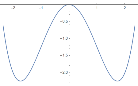
One or both of the following plots may be what you looking for.

α = 1;
β = 1;
Tmp = 0.1316;
ρ = 0.01;
T = -2;

FreeEnergy = 
  1/2*(T - 1)*P^2 + 
   1/4*P^4 + (1/2*α^2*β*M^2*(T - Tmp)) + 
   1/4 α^2*(β)*(M^4) + 1/2*(ρ*(P^2)*(M^2));

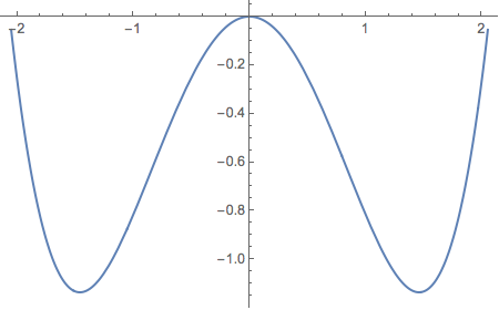
Plot[Evaluate[FreeEnergy /. M -> 0], {P, -2.35669, 2.35669}]

plot1

Plot[Evaluate[FreeEnergy /. P -> 0], {M, -2.05216, 2.05217}]

plot2

$\endgroup$
1
$\begingroup$

After help from everybody. this question has been resolved. we can do as follows;

α= 1;
β= 1;
tmp = 0.1316;
ρ= 0.01;
t = -2;

fe[m_, p_] := 
 1/2*(t - 1)*p^2 + 1/4*p^4 + (1/2*α^2*β*m^2*(t - tmp)) + 
  1/4 α^2*(β)*(m^4) + 1/2*(ρ*(p^2)*(m^2))

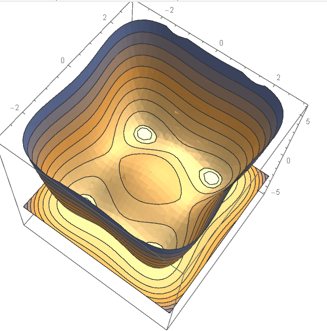
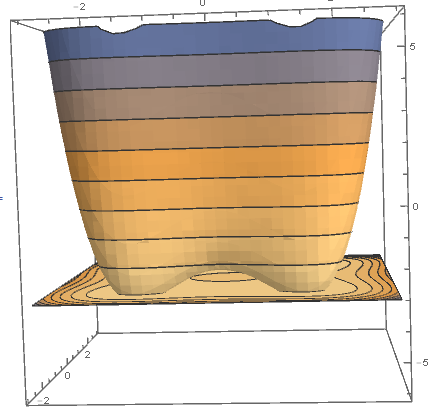
Show[SliceContourPlot3D[
  z - fe[m, p], {z == -3}, {m, -3, 3}, {p, -3, 3}, {z, -6, 6}], 
 SliceContourPlot3D[-z, 
  z == fe[m, p], {m, -3, 3}, {p, -3, 3}, {z, -6, 6}]]

Top view

Side view

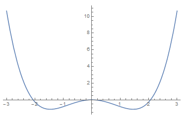
Plot[Evaluate[FreeEnergy /. P -> 0], {M, -3, 3}]

2-D

$\endgroup$

Your Answer

By clicking “Post Your Answer”, you agree to our terms of service and acknowledge you have read our privacy policy.

Not the answer you're looking for? Browse other questions tagged or ask your own question.