How to discretize a nonlinear PDE fast?

Question

I wish to numerically solve the following PDE. Although there are some complete discussions for solving PDEs in tutorial/NDSolvePDE, there is no hint for the nonlinear case by discretization. Thus, I will be thankful to receive some helps on the following NPDE where $x \in [0,1]$, $t \in [0,2]$,

The equation is

$$\frac{\partial u(x,t)}{\partial t}+u(x,t) \frac{\partial u(x,t)}{\partial x}=c \frac{\partial ^2u(x,t)}{\partial x^2}$$

with initial condition

$$u(x,0)=\frac{2 \pi \beta c \sin (\pi x)}{\alpha +\beta \cos (\pi x)}$$

and boundary conditions

$$u(0,t)=u(1,t)=0$$

I tried the backward finite difference (FD) for $\frac{\partial u(x,t)}{\partial t}$ and the central FD for the others. I wrote the following code, but I think there are some gaps in it. Because, the approximate solutions do not match the exact one

$$u(x,t)=\frac{2 \pi \beta c e^{-c \pi ^2 t} \sin (\pi x)}{\alpha +\beta e^{-c \pi ^2 t} \cos (\pi x)}$$

Note that Subscript[w, i, j] stands for the approximation in the grid point $(x_i,t_j)$.

M = 8; NN = 8; m = M - 1; 
n = NN - 1; alpha = 5.; 
beta = 4.; c = 0.05; 
T = 2.; h = (1. - 0.)/M; 
k =T/NN;

(*Defining the Grid points*)
Table[Subscript[x, i] = 0 + i h, {i, 0, M}]; 
Table[Subscript[t, j] = 0 + j k, {j, 0, NN}];

(*Defining the Initial Conditions*)
For[i = 1, i <= m, i++, 
  Subscript[w, i, 0] = (2. c beta Pi Sin[Pi Subscript[x, i]])
                     / (alpha + beta Cos[Pi Subscript[x, i]])
];

(*Defining the Boundary Conditions*)
For[j = 1, j <= n, j++, 
  Subscript[w, 0, j] = 0
]; 
For[j = 1, j <= n, j++, 
  Subscript[w, 1, j] = 0
];

(*Defining the nonlinear equations due to discretization*)
For[i = 1, i <= m, i++,
  {
   For[j = 1, j <= n, j++,
     f[i, j] = Subscript[w, i, j] 
       + (k/(2 h)) Subscript[w, i, j] (Subscript[w, i + 1, j] - Subscript[w, i - 1, j]) 
       - (c k/(h^2)) (Subscript[w, i + 1, j] - 2 Subscript[w, i, j] 
                      + Subscript[w, i - 1, j]) 
       - Subscript[w,i, j - 1]
   ]
  }
];

F = Flatten[Table[f[i, j], {i, 1, m}, {j, 1, n}]]; 
Dimensions[F];
F // MatrixForm;
Vec = Flatten[Table[Subscript[w, i, j], {i, 2, M}, {j, 1, n}]];

(*Finding the solutions*)
Sol = Part[NSolve[F, Vec, Reals], 1]

Any suggestion is appreciated. In fact, what would be the final nonlinear system of equations resulting of discretization?

Answer 1

These days I've picked up some knowledge about finite difference method and now I'm able to fix OP's code :D.

Well, before beginning, it should be mentioned that, it's better to avoid For and Subscript in Mathematica, but I'd rather not talk about them in this answer since these have been discussed a lot in this site, what's more, they're not the root of the "gap" in OP's code. To fix the code, there're two major issues:

1. Something is wrong with the indices of the grid points

In the following part of the code, you lose 4 grid points and mix up the indices of the grid points and the real coordinates when defining IC and BC:

(*Defining the Initial Conditions*) 
For[i = 1, i <= m, i++, 
    Subscript[w, i, 0] = 
        (2. c beta Pi Sin[Pi Subscript[x, i]])/(alpha + beta Cos[Pi Subscript[x, i]])];
(*Defining the Boundary Conditions*) 

For[j = 1, j <= n, j++, Subscript[w, 0, j] = 0]

For[j = 1, j <= n, j++, Subscript[w, 1, j] = 0]

You've divided the domain into 8*8 equal parts, so just as the following graph illustrates:

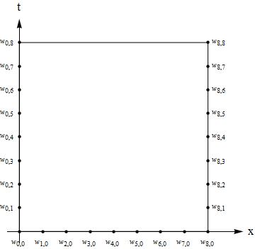
j is actually from 0 to NN:

For[j = 0, j <= NN, j++, Subscript[w, 0, j] = 0]
For[j = 0, j <= NN, j++, Subscript[w, M(* Notice here! *), j] = 0]

Similar mistakes lie in the definition of f[i, j] and F and Vec:

For[i = 1, i <= m, i++, {For[j = 1, j <= n, j++, f[i, j] = Subscript[w, i, j] + (k/(2 h)) Subscript[w, i, j] (Subscript[w, i + 1, j] - Subscript[w, i - 1, j]) - (c k/(h^2)) (Subscript[w, i + 1, j] - 2 Subscript[w, i, j] + Subscript[w, i - 1, j]) - Subscript[w, i, j - 1]]}];

The j <= n should be j <= NN:

For[i = 1, i <= m, 
  i++, {For[j = 1, j <= NN, j++, 
    f[i, j] = 
     Subscript[w, i, 
       j] + (k/(2 h)) Subscript[w, i, 
        j] (Subscript[w, i + 1, j] - 
         Subscript[w, i - 1, j]) - (c k/(h^2)) (Subscript[w, i + 1, 
          j] - 2 Subscript[w, i, j] + Subscript[w, i - 1, j]) - 
      Subscript[w, i, j - 1]]}];

F = Flatten[Table[f[i, j], {i, 1, m}, {j, 1, n}]];

Vec = Flatten[Table[Subscript[w, i, j], {i, 2, M}, {j, 1, n}]];

Fixed version:

F = Flatten[Table[f[i, j], {i, m}, {j, NN}]];
Vec = Flatten[Table[Subscript[w, i, j], {i, m}, {j, NN}]];

2. How to solve the set of equations faster

Once we finish the modifications above, we can get the correct solution in principle, while the real trouble starts in fact… as mentioned in the comments above, the result of using backward finite difference together with central finite difference is, we need $w_{i-1,j}, w_{i+1,j}, w_{i,j-1}$ to get $w_{i,j}$ i.e. there are always 2 or more than 2 unknown variables in the difference formula, as shown in the GIF below:

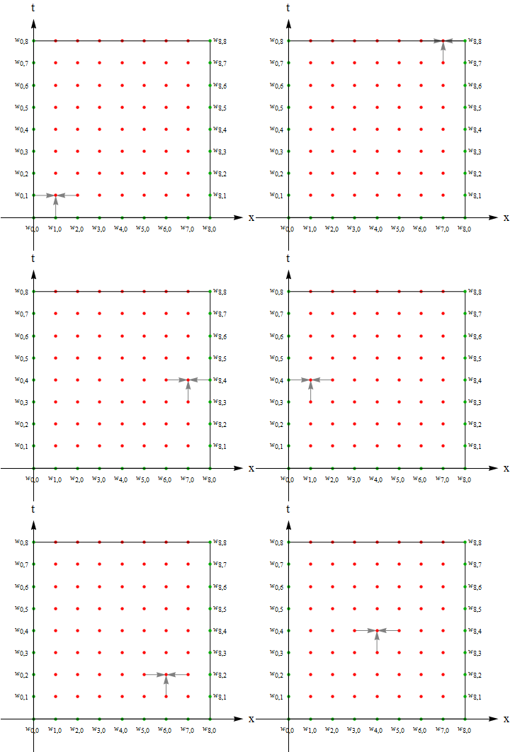
Green points for the knowns, red points for the unknowns and gray arrows for the difference formula, no matter where you put the three arrows, there're 2 or more than 2 unknown points.

So "simple" iteration(as PlatoManiac has tried in his answer) won't work in this case because it causes endless loop. (for example, to get $w_{1,1}$, Mathematica calls $w_{0,1}, w_{2,1}, w_{1,0}$, but $w_{2,1}$ is unknown, so Mathematica goes on calling $w_{1,1}, w_{3,1}, w_{2,0}$: $w_{1,1}$ is called again! Then it never finishes… )

Of course, all these equations form a closed equation groups, it can be solved theoretically, and that's what you've tried in your code, but solving this set of equations (for your case you need to solve 56 interrelated quadratic equations…) with Solve or NSolve is extremely slow. (Your original code is fast because of the mistakes I mentioned above… )

We need a work-around.

One choice is to use FindRoot instead, though FindRoot often disappoints me, it really works well for your equation:

Sol = FindRoot[F, {#, 1} & /@ Vec];
Table[Subscript[w, i, j], {i, 0, M}, {j, 0, NN}] /. Sol;
solFD = ListInterpolation[%, {{0, 1}, {0, 2}}];
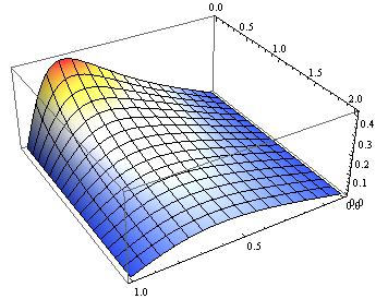
Plot3D[solFD[x, t], {x, 0, 1}, {t, 0, 2}]

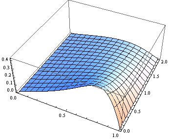
Let's compare it to the analytical solution:

α = 5.; β = 4.; c = 0.05;
u[x_, t_] := (2 β c Pi Exp[-c Pi^2 t] Sin[Pi x])/(α + β Exp[-c Pi^2 t] Cos[Pi x]);
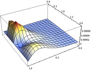
Plot3D[solFD[x, t] - u[x, t], {x, 0, 1}, {t, 0, 2}]

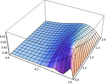
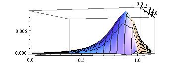
Hmm… not bad, considering the sparse grid. By the way, if we increase M and N, for example, to:

M = 25; NN = 25;

The error will decrease to:

Another approach is to use the classic relaxation method, to make the implementation of the algorithm conciser, I'd like to have some big changes on your original code.

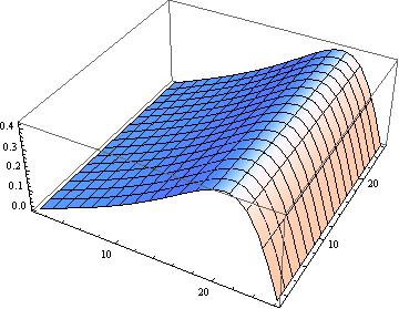
First, we need to acquire the initial guess of the solution, A better guess can improve the speed of convergence, but here I simply choose IC just for convenience:

m = 25; n = 25;
α = 5.; β = 4.; c = 0.05;
x1 = 0.; x2 = 1.; t1 = 0.; t2 = 2.;
dx = (x2 - x1)/m;
dt = (t2 - t1)/n;
int = Table[(2 β c Pi Sin[Pi i dx])/(α + β Cos[Pi i dx]), {i, 0, m}, {j, 0, n}];
ListPlot3D[int\[Transpose]]

The initial guess:

Also, the explicit expression of difference formula is necessary, here I define it as a function:

mid[u_, i_, j_] = 
  Quiet[u[[i, j]] /. 
    First@Solve[
      u[[i, j]] + (dt/(2 dx)) u[[i, j]] (u[[i + 1, j]] - 
           u[[i - 1, j]]) - (c dt/(dx^2)) (u[[i + 1, j]] - 
           2 u[[i, j]] + u[[i - 1, j]]) - u[[i, j - 1]] == 0, u[[i, j]]]];

OK, let's iterate!:

list = FixedPoint[
    Table[If[i == 0 || i == m || j == 0, #[[i + 1, j + 1]], 
       mid[#, i + 1, j + 1]], {i, 0, m}, {j, 0, n}] &, int, 
    SameTest -> (Max[Abs[#2 - #1]] < 0.0001 &)]; // AbsoluteTiming

{2.5216000, Null}

Remark: Though not that important in this problem, using the experience got in this and this post, we can speed up the iteration:

iter = ReleaseHold[
    Hold@Compile[{{int, _Real, 2}}, 
        Module[{d = Dimensions@int}, 
         FixedPoint[
          Table[If[i == 1 || i == d[[1]] || j == 1, #[[i, j]], 
             mid[#, i, j]], {i, d[[1]]}, {j, d[[2]]}] &, int, 
          SameTest -> (Max[Abs[#2 - #1]] < 0.0001 &)]], 
        CompilationTarget -> "C", RuntimeOptions -> "Speed"] /. 
      DownValues@mid /. Part -> Compile`GetElement]; 

list = iter@int; // AbsoluteTiming

{0.0030000, Null}

Remember to take away the CompilationTarget -> "C", if you don't have a C compiler installed, and notice that iter can actually accept any initial guess.

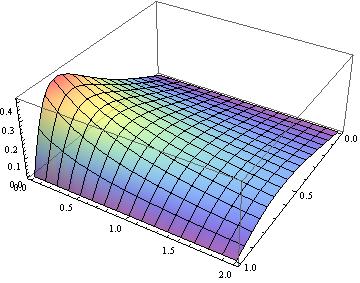
Here's the result:

solRe = ListInterpolation[list, {{0, 1}, {0, 2}}];
Plot3D[solRe[x, t], {x, 0, 1}, {t, 0, 2}, ColorFunction->"Rainbow", PlotStyle->Opacity[2/3]]

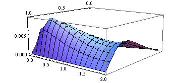
Error check:

u[x_, t_] := (2 β c Pi Exp[-c Pi^2 t] Sin[Pi x])/(α + β Exp[-c Pi^2 t] Cos[Pi x]);
Plot3D[solRe[x, t] - u[x, t], {x, 0, 1}, {t, 0, 2}, PlotRange -> All]

Finally, we understand how cute our NDSolve is:

Clear[u, v]
a = 5; b = 4; c = 1/20;
t1 = 0; t2 = 2; x1 = 0; x2 = 1;

sol = NDSolve[{D[u[x, t], t] + u[x, t] D[u[x, t], x] == c D[u[x, t], x, x], 
               u[x, 0] == (2 b c Pi Sin[Pi x])/(a + b Cos[Pi x]), 
               u[0, t] == u[1, t] == 0}, u, {x, x1, x2}, {t, t1, t2}];

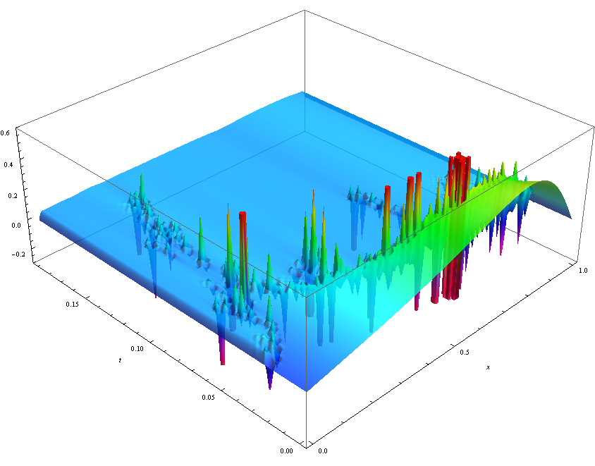
Plot3D[u[x, t] /. sol, {x, x1, x2}, {t, t1, t2}, ColorFunction -> "TemperatureMap"]

v[x_, t_] := (2 c b Pi Exp[-c Pi^2 t] Sin[Pi x])/(a + b Exp[-c Pi^2 t] Cos[Pi x]);
Plot3D[(u[x, t] /. sol) - v[x, t], {x, x1, x2}, {t, t1, t2}, 
       ColorFunction -> "TemperatureMap"]

Answer 2

A quick answer now. I will come back to this once I have more time. First we use the common finite difference operators to discretize PDE.

Symbolics:

Clear[u];
RFSDiscrit[eq_] := 
Module[{mid},
       mid = Distribute@FullSimplify@ExpandAll[(
        eq /.{
          u[x, t] -> u[i, n],
          D[u[x, t], t] -> (u[i, n] - u[i, n - 1])/\[CapitalDelta]t,
          D[u[x, t], x, x] ->
          (u[i + 1, n - 1] - 2 u[i, n - 1] + u[i - 1, n - 1])/\[CapitalDelta]x^2
             }
        )];
       (First@Solve[mid == 0, u[i, n]])[[All, 2]] // First
       ];

Recursion:

Lets generate the recursive formula for the main equation.

exp = RFSDiscrit[D[u[x, t], t] + (c - u[x, t]) D[u[x, t], x, x]]

Now comes the rest of the recursion definition part.

alpha = 5.;
beta = 4.;
c = .05;
(*Use recursive formula*)
u[i_, n_] := u[i, n] = exp;
u[0, n_] := u1[t] /. t -> n \[CapitalDelta]t;
(*Number of discretization points for [0,L]*)
spacediscrit = 100; 
u[spacediscrit, n_] := u2[t] /. t -> n \[CapitalDelta]t;
u[i_, 0] := u0[x] /. x -> i \[CapitalDelta]x;
(* End of spatial boundary*)
L = 1;
timesteps = 1000;
\[CapitalDelta]t = 2/timesteps;
\[CapitalDelta]x = L/spacediscrit;
(*Initial Condition*)
u0[x_] = (2. c beta Pi Sin[Pi x])/(alpha + beta Cos[Pi x]);
(*Boundary Condition*)
u1[t_] = 0;
u2[t_] = 0;
(* Time snapshots for u(x,t_n)*)
pics = Table[ListPlot[Table[{\[CapitalDelta]x i, u[i, n]},{i, 0, spacediscrit}], 
            InterpolationOrder -> 3, Joined -> True, Mesh -> 10, 
            MeshStyle -> Red, Filling -> Axis, FillingStyle -> LightPink, 
            Frame -> True, PlotRange -> All, Axes -> None, 
            PlotLabel ->TraditionalForm[
             "u(x,t) at t=" <>ToString[\[CapitalDelta]t n // N]]
             ], 
            {n, 0, timesteps,30}];

Good/Bad-ness of...!

Now we can get $u(x,t)$ as a continuous function as follows.

dat = Table[Table[N@{\[CapitalDelta]x j, \[CapitalDelta]t n, u[j, n]}, 
            {j, 0,spacediscrit}],
      {n, 0, timesteps}];
fun = Interpolation[Flatten[dat, 1]]

InterpolatingFunction[{{0.,1.},{0.,2.}},<>]

Now a nice plot to celebrate the nasty numerical instability of the above equation on the given parameter setting.

The MMA function NDSolve FiniteDifferenceDerivative can also be used for discretization.

Answer 3

From version 12.0 onward you can solve this with the finite element method. In fact there is a closely related example in the nonlinear FEM verification tests that are part of the FEM documentation. Specifically I am talking about the FEM-NL-Transient-1D-Single-Convection-0002 test. It's better to read in the documentation under FEMDocumentation/tutorial/NonlinearFiniteElementVerificationTests#658234114.

Here is the code:

Clear[u, v]
a = 5; b = 4; c = 1/20;
t1 = 0; t2 = 2; x1 = 0; x2 = 1;

sol = NDSolve[{D[u[x, t], t] + u[x, t] D[u[x, t], x] == 
     c D[u[x, t], x, x], 
    u[x, 0] == (2 b c Pi Sin[Pi x])/(a + b Cos[Pi x]), 
    u[0, t] == u[1, t] == 0}, u, {x, x1, x2}, {t, t1, t2}, 
   Method -> {"MethodOfLines", 
     "SpatialDiscretization" -> {"FiniteElement"}}];

Plot3D[u[x, t] /. sol, {x, x1, x2}, {t, t1, t2}, 
 ColorFunction -> "TemperatureMap"]