3
$\begingroup$

I'm trying to solve numerically the following system in a rectangular region,

$\begin{align} \cos\theta\frac{\partial\beta}{\partial x}+\sin\theta\frac{\partial\beta}{\partial y}&=\beta s\\-\sin\theta\frac{\partial\alpha}{\partial x}+\cos\theta\frac{\partial\alpha}{\partial y}&=-\alpha b\\\cos\theta\frac{\partial s}{\partial x}+\sin\theta\frac{\partial s}{\partial y}&=-s^{2}\\-\sin\theta\frac{\partial b}{\partial x}+\cos\theta\frac{\partial b}{\partial y}&=b^{2}\\ \cos\theta\frac{\partial\theta}{\partial x}+\sin\theta\frac{\partial\theta}{\partial y}&=b \end{align}$

subject to initial conditions along an arbitrary line in the $x,y$ plane. To begin with I use the $x$ axis:

$\theta(x,0)=x^2, \frac{\partial\theta(x,0)}{\partial y}=x,\:s(x,0)=\cos x,\:\alpha(x,0)=\beta(x,0)=1,\:b(x,0)=\cos\theta(x,0)\frac{\partial\theta(x,0)}{\partial x}+\sin\theta(x,0)\frac{\partial\theta(x,0)}{\partial y}$

But mathematica is not returning anything, the solutions just satisfy the conditions and then drop to zero. I get the following warnings:

NDSolveFEMInitializePDECoefficients::femcscd: The PDE is convection dominated and the result may not be stable. Adding artificial diffusion may help.

NDSolveFEMInitializePDECoefficients::femcscd: The PDE is convection dominated and the result may not be stable. Adding artificial diffusion may help.

FindRoot::stfail: The method AffineCovariantNewton failed to compute the next step.

FindRoot::sszero: The step size in the search has become less than the tolerance prescribed by the PrecisionGoal option, but the function value is still greater than the tolerance prescribed by the AccuracyGoal option.

I don't have any clue what's the matter with NDSolve.

Thank you so much for any help.

The code:

region = Rectangle[{0, 0}, {0.5, 0.5}];
eq1 = Cos[θ[x, y]] D[β[x, y], x] + 
    Sin[θ[x, y]] D[β[x, y], y] == β[x, y] s[x, y];
eq2 = -Sin[θ[x, y]] D[α[x, y], x] + 
    Cos[θ[x, y]] D[α[x, y], y] == -α[x, y] b[x, 
     y];
eq3 = Cos[θ[x, y]] D[s[x, y], x] + 
    Sin[θ[x, y]] D[s[x, y], y] == -s[x, y]^2;
eq4 = -Sin[θ[x, y]] D[b[x, y], x] + 
    Cos[θ[x, y]] D[b[x, y], y] == b[x, y]^2;
eq5 = Cos[θ[x, y]] D[θ[x, y], x] + 
    Sin[θ[x, y]] D[θ[x, y], y] == b[x, y];
bc = {θ[x, 0] == x^2,
   β[x, 0] == 1,
   α[x, 0] == 1,
   s[x, 0] == Cos[x],
   b[x, 0] == 2 x Cos[x^2] + Sin[x^2] x};

sol = NDSolve[{{eq1, eq2, eq3, eq4, eq5}, bc}, {α, β, b, 
    s, θ}, {x, y} ∈ region];

When plotting the solutions I get things like

enter image description here

$\endgroup$
6
  • 1
    $\begingroup$ The help has some information about this: have a look at FEMDocumentation/ref/message/InitializePDECoefficients/femcscd $\endgroup$
    – user21
    Commented Dec 16, 2020 at 14:50
  • $\begingroup$ The way you have posed your problem is that there is no driving force in the y-direction. All your BCs are either constant or depend only on x. The y-derivatives in your equations should vanish. A diffusive term or a flux boundary condition would drive some flow in the y-direction. $\endgroup$
    – Tim Laska
    Commented Dec 16, 2020 at 22:47
  • $\begingroup$ I'm not sure if I understand your remark. The BCs of course only depend on x because they are given along a y-constant line. Like in the wave equation, you specify the initial profile and velocity at t=0, the BCs doesn't depend on t. $\endgroup$ Commented Dec 17, 2020 at 8:58
  • $\begingroup$ If you are replying to me, you need to start with the@TimLaska so that I am notified of your reply. The wave equation has a second-order time derivative plus a second-order spatial derivative (a diffusive or Laplacian term). You only have first-order spatial or convective terms. $\endgroup$
    – Tim Laska
    Commented Dec 17, 2020 at 15:26
  • 1
    $\begingroup$ Version 13 has ToGradedMesh and ElementMeshRegionProduct. $\endgroup$
    – user21
    Commented Dec 16, 2021 at 8:06

2 Answers 2

5
$\begingroup$

This is an extended comment versus an answer. Following @user21's link, it suggests refining the mesh at the boundaries. The features are very sharp at the Y = 0 boundary. I am going to apply anisotropic meshing and attempt to capture the features. Furthermore, I'm going to shrink the y-dimension since the solution falls off very quickly.

Helper functions

To create the anisotropic mesh, I will first find some helper functions:

(*Import required FEM package*)
Needs["NDSolve`FEM`"];
(* Define Some Helper Functions For Structured Quad Mesh*)
pointsToMesh[data_] :=
  MeshRegion[Transpose[{data}], 
   Line@Table[{i, i + 1}, {i, Length[data] - 1}]];
unitMeshGrowth[n_, r_] := 
 Table[(r^(j/(-1 + n)) - 1.)/(r - 1.), {j, 0, n - 1}]
meshGrowth[x0_, xf_, n_, r_] := (xf - x0) unitMeshGrowth[n, r] + x0
firstElmHeight[x0_, xf_, n_, r_] := 
 Abs@First@Differences@meshGrowth[x0, xf, n, r]
lastElmHeight[x0_, xf_, n_, r_] := 
 Abs@Last@Differences@meshGrowth[x0, xf, n, r]
findGrowthRate[x0_, xf_, n_, fElm_] := 
 Quiet@Abs@
   FindRoot[firstElmHeight[x0, xf, n, r] - fElm, {r, 1.0001, 100000}, 
     Method -> "Brent"][[1, 2]]
meshGrowthByElm[x0_, xf_, n_, fElm_] := 
 N@Sort@Chop@meshGrowth[x0, xf, n, findGrowthRate[x0, xf, n, fElm]]
meshGrowthByElm0[len_, n_, fElm_] := meshGrowthByElm[0, len, n, fElm]
flipSegment[l_] := (#1 - #2) & @@ {First[#], #} &@Reverse[l];
leftSegmentGrowth[len_, n_, fElm_] := meshGrowthByElm0[len, n, fElm]
rightSegmentGrowth[len_, n_, fElm_] := Module[{seg},
  seg = leftSegmentGrowth[len, n, fElm];
  flipSegment[seg]
  ]
reflectRight[pts_] := With[{rt = ReflectionTransform[{1}, {Last@pts}]},
  Union[pts, Flatten[rt /@ Partition[pts, 1]]]]
reflectLeft[pts_] := 
 With[{rt = ReflectionTransform[{-1}, {First@pts}]},
  Union[pts, Flatten[rt /@ Partition[pts, 1]]]]
extendMesh[mesh_, newmesh_] := Union[mesh, Max@mesh + newmesh]

Create an isotropic Quad mesh

I'm going to shrink the y-dimension to ${10^{ - 7}}$ and have a growth rate where the first element is a thousand times smaller than the last element.

seg = Subdivide[0, 0.5, 40];
Print["Horizontal segment"]
rh = pointsToMesh@seg
seg = leftSegmentGrowth[0.0000001, 100, 0.0000001/1000];
Print["Vertical segment"]
rv = pointsToMesh@seg
(*View Region Product of horiz and vert segs*)
Print["2D Region via RegionProduct"]
rp = RegionProduct[rh, rv]
(*Extract Coords from RegionProduct*)
crd = MeshCoordinates[rp];
(*grab quad element incidents RegionProduct mesh*)
inc = Delete[0] /@ MeshCells[rp, 2];
(mesh = ToElementMesh["Coordinates" -> crd, 
    "MeshElements" -> {QuadElement[inc]}])["Wireframe"]
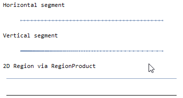
Then 2D mesh

Solve and plot the solutions

eq1 = Cos[θ[x, y]] D[β[x, y], x] + 
    Sin[θ[x, y]] D[β[x, y], y] == β[x, y] s[x, y];
eq2 = -Sin[θ[x, y]] D[α[x, y], x] + 
    Cos[θ[x, y]] D[α[x, y], y] == -α[x, y] b[x, 
     y];
eq3 = Cos[θ[x, y]] D[s[x, y], x] + 
    Sin[θ[x, y]] D[s[x, y], y] == -s[x, y]^2;
eq4 = -Sin[θ[x, y]] D[b[x, y], x] + 
    Cos[θ[x, y]] D[b[x, y], y] == b[x, y]^2;
eq5 = Cos[θ[x, y]] D[θ[x, y], x] + 
    Sin[θ[x, y]] D[θ[x, y], y] == b[x, y];
bc = {θ[x, 0] == x^2, β[x, 0] == 1, α[x, 0] == 1, 
   s[x, 0] == Cos[x], b[x, 0] == 2 x Cos[x^2] + Sin[x^2] x};
{αfun, βfun, bfun, sfun, θfun} = 
  NDSolveValue[{{eq1, eq2, eq3, eq4, eq5}, bc}, {α, β, b,
     s, θ}, {x, y} ∈ mesh];
{αfun, βfun, bfun, sfun, θfun} = 
  NDSolveValue[{{eq1, eq2, eq3, eq4, eq5}, bc}, {α, β, b,
     s, θ}, {x, y} ∈ mesh];
Plot3D[αfun[x, y], {x, y} ∈ mesh, PlotPoints -> All, 
 ViewPoint -> Right]
Plot3D[βfun[x, y], {x, y} ∈ mesh, PlotPoints -> All, 
 ViewPoint -> Right]
Plot3D[bfun[x, y], {x, y} ∈ mesh, PlotPoints -> All, 
 ViewPoint -> Right]
Plot3D[sfun[x, y], {x, y} ∈ mesh, PlotPoints -> All, 
 ViewPoint -> Right]
Plot3D[θfun[x, y], {x, y} ∈ mesh, PlotPoints -> All, 
 ViewPoint -> Right]
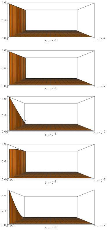
No diffusive term solution

As you can see, nothing gets pulled off the Y = 0 boundary, even at incredible resolution.

Add a diffusive term to the full domain

seg = Subdivide[0, 0.5, 40];
Print["Horizontal segment"]
rh = pointsToMesh@seg
seg = leftSegmentGrowth[0.5, 100, 0.5/1000];
Print["Vertical segment"]
rv = pointsToMesh@seg
(*View Region Product of horiz and vert segs*)
Print["2D Region via RegionProduct"]
rp = RegionProduct[rh, rv]
(*Extract Coords from RegionProduct*)
crd = MeshCoordinates[rp];
(*grab quad element incidents RegionProduct mesh*)
inc = Delete[0] /@ MeshCells[rp, 2];
Print["Element mesh"]
(mesh = ToElementMesh["Coordinates" -> crd, 
    "MeshElements" -> {QuadElement[inc]}])["Wireframe"]
(*Artificial diffusion constant*)
cart = 10^-3
eq1 = Cos[θ[x, y]] D[β[x, y], x] + 
    Sin[θ[x, y]] D[β[x, y], y] + 
    Div[-cart Grad[β[x, y], {x, y}], {x, y}] == β[x, y] s[
     x, y];
eq2 = -Sin[θ[x, y]] D[α[x, y], x] + 
    Cos[θ[x, y]] D[α[x, y], y] + 
    Div[-cart Grad[α[x, y], {x, y}], {x, y}] == -α[x, 
      y] b[x, y];
eq3 = Cos[θ[x, y]] D[s[x, y], x] + 
    Sin[θ[x, y]] D[s[x, y], y] + 
    Div[-cart Grad[s[x, y], {x, y}], {x, y}] == -s[x, y]^2;
eq4 = -Sin[θ[x, y]] D[b[x, y], x] + 
    Cos[θ[x, y]] D[b[x, y], y] + 
    Div[-cart Grad[b[x, y], {x, y}], {x, y}] == b[x, y]^2;
eq5 = Cos[θ[x, y]] D[θ[x, y], x] + 
    Sin[θ[x, y]] D[θ[x, y], y] + 
    Div[-cart Grad[θ[x, y], {x, y}], {x, y}] == b[x, y];
bc = {θ[x, 0] == x^2, β[x, 0] == 1, α[x, 0] == 1, 
   s[x, 0] == Cos[x], b[x, 0] == 2 x Cos[x^2] + Sin[x^2] x};
{αfun, βfun, bfun, sfun, θfun} = 
  NDSolveValue[{{eq1, eq2, eq3, eq4, eq5}, bc}, {α, β, b,
     s, θ}, {x, y} ∈ mesh];
{αfun, βfun, bfun, sfun, θfun} = 
  NDSolveValue[{{eq1, eq2, eq3, eq4, eq5}, bc}, {α, β, b,
     s, θ}, {x, y} ∈ mesh];
Print["Plot of solutions"]
Plot3D[αfun[x, y], {x, y} ∈ mesh, PlotPoints -> All, 
 PlotRange -> All, ViewPoint -> Right]
Plot3D[βfun[x, y], {x, y} ∈ mesh, PlotPoints -> All, 
 PlotRange -> All, ViewPoint -> Right]
Plot3D[bfun[x, y], {x, y} ∈ mesh, PlotPoints -> All, 
 PlotRange -> All, ViewPoint -> Right]
Plot3D[sfun[x, y], {x, y} ∈ mesh, PlotPoints -> All, 
 PlotRange -> All, ViewPoint -> Right]
Plot3D[θfun[x, y], {x, y} ∈ mesh, PlotPoints -> All, 
 PlotRange -> All, ViewPoint -> Right]

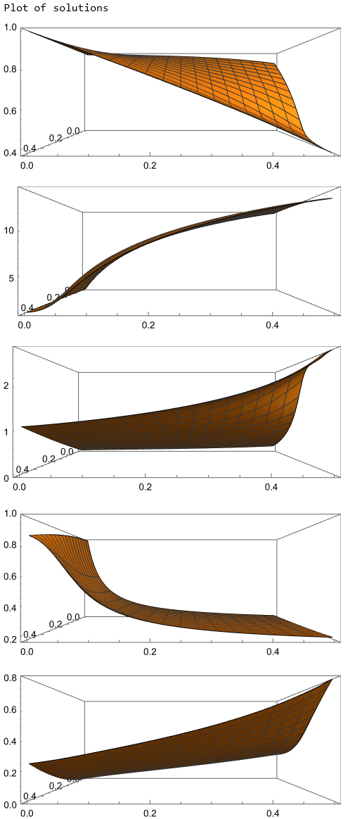
Solutions with artificial diffusion

As you can see, an explicit diffusive term will pull material into the domain from the boundary.

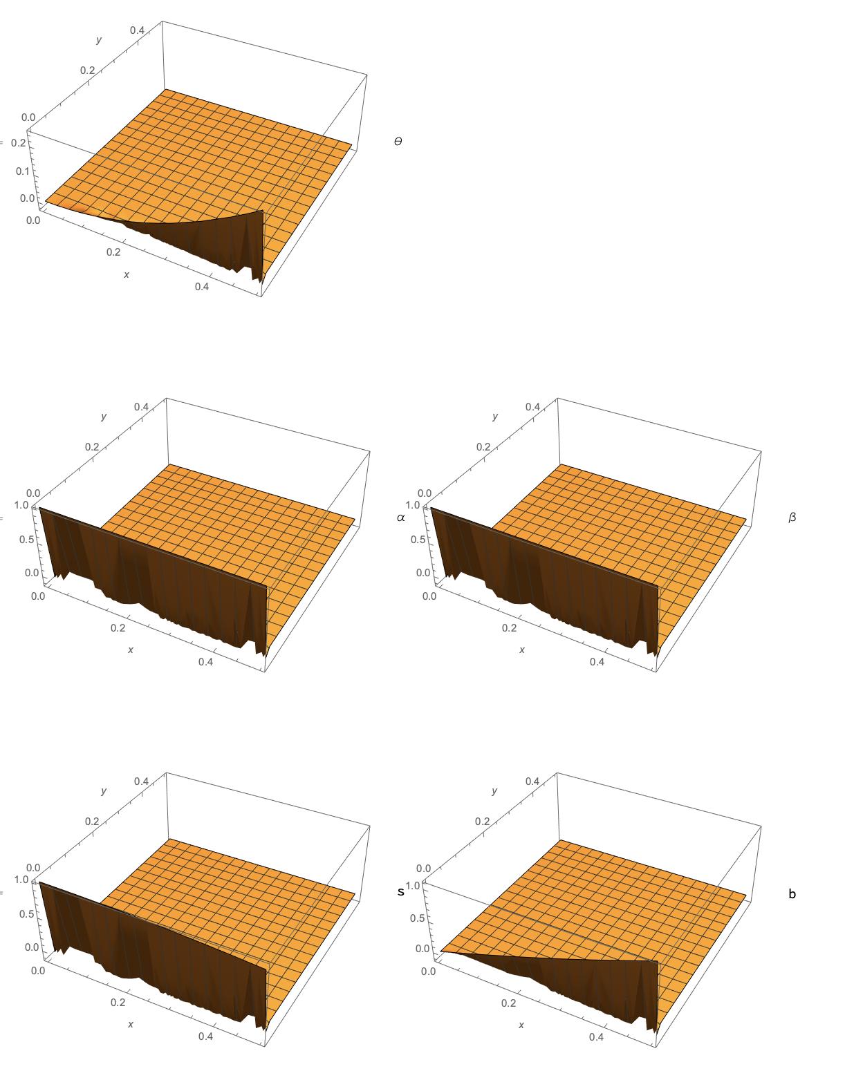
$\endgroup$
1
  • $\begingroup$ @Daniel Castro, Tim made a proposal to add anisotropic meshing capabilities to the FEM mesh generation here. If you think this is worthwhile, consider giving this proposal an upvote $\endgroup$
    – user21
    Commented Feb 22, 2021 at 10:34
5
$\begingroup$

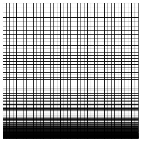
This is the same approach that Tim describes in his solution, but implemented with the ToGradedMesh and ElementMeshRegionProduct functions added in version 13.0:

meshX = ToGradedMesh[Line[{{0}, {0.5}}], <|"ElementCount" -> 40|>];
meshY = ToGradedMesh[Line[{{0}, {0.5}}],
    <|"Alignment" -> "Left",
    "ElementCount" -> 100, 
    "MinimalDistance" -> 0.5/1000|>
];

MeshRegion /@ {meshX, meshY}

meshXY

mesh = ElementMeshRegionProduct[meshX, meshY];
mesh["Wireframe"]

mesh

cart = 10^-3;
eq1 = Cos[θ[x, y]] D[β[x, y], x] + 
    Sin[θ[x, y]] D[β[x, y], y] + 
    Div[-cart Grad[β[x, y], {x, y}], {x, y}] == β[x, y] s[
     x, y];
eq2 = -Sin[θ[x, y]] D[α[x, y], x] + 
    Cos[θ[x, y]] D[α[x, y], y] + 
    Div[-cart Grad[α[x, y], {x, y}], {x, y}] == -α[x, 
      y] b[x, y];
eq3 = Cos[θ[x, y]] D[s[x, y], x] + 
    Sin[θ[x, y]] D[s[x, y], y] + 
    Div[-cart Grad[s[x, y], {x, y}], {x, y}] == -s[x, y]^2;
eq4 = -Sin[θ[x, y]] D[b[x, y], x] + 
    Cos[θ[x, y]] D[b[x, y], y] + 
    Div[-cart Grad[b[x, y], {x, y}], {x, y}] == b[x, y]^2;
eq5 = Cos[θ[x, y]] D[θ[x, y], x] + 
    Sin[θ[x, y]] D[θ[x, y], y] + 
    Div[-cart Grad[θ[x, y], {x, y}], {x, y}] == b[x, y];
bc = {θ[x, 0] == x^2, β[x, 0] == 1, α[x, 0] == 1, 
   s[x, 0] == Cos[x], b[x, 0] == 2 x Cos[x^2] + Sin[x^2] x};
{αfun, βfun, bfun, sfun, θfun} = 
  NDSolveValue[{{eq1, eq2, eq3, eq4, eq5}, bc}, {α, β, b,
     s, θ}, {x, y} ∈ mesh];
{αfun, βfun, bfun, sfun, θfun} = 
  NDSolveValue[{{eq1, eq2, eq3, eq4, eq5}, bc}, {α, β, b,
     s, θ}, {x, y} ∈ mesh];
Print["Plot of solutions"]
Plot3D[αfun[x, y], {x, y} ∈ mesh, PlotPoints -> All, 
 PlotRange -> All, ViewPoint -> Right]
Plot3D[βfun[x, y], {x, y} ∈ mesh, PlotPoints -> All, 
 PlotRange -> All, ViewPoint -> Right]
Plot3D[bfun[x, y], {x, y} ∈ mesh, PlotPoints -> All, 
 PlotRange -> All, ViewPoint -> Right]
Plot3D[sfun[x, y], {x, y} ∈ mesh, PlotPoints -> All, 
 PlotRange -> All, ViewPoint -> Right]
Plot3D[θfun[x, y], {x, y} ∈ mesh, PlotPoints -> All, 
 PlotRange -> All, ViewPoint -> Right]

solutions

$\endgroup$

Your Answer

By clicking “Post Your Answer”, you agree to our terms of service and acknowledge you have read our privacy policy.