10
$\begingroup$

An interesting issue was raised in comments to the following question: Monitoring Plot3D with a given number of plotpoints.

We were discussing the fact that a Plot3D expression with options PlotPoints -> points and MaxRecursion -> 0 evaluated the function to be plotted $4 \ \textrm{points}^2$, instead of simply $\textrm{points}^2$ times as I would have expected from the documentation. In fact, the docs for PlotPoints state that, with more than one variable, PlotPoints -> n specifies that $n$ initial points should be used in each direction. That, together with the MaxRecursion -> 0 should stop any attempts at further refinement.

Searching this site, I learned that the extra evaluations are used to calculate the "vertex normals" (see Why does Plot3D appear to traverse the points twice? and Henrik's answer there). This can be turned off using NormalsFunction -> None.

At first, however, I did not know about NormalsFunction and its effect, so I was playing around with a toy example, and I noticed a pattern in the function evaluations within Plot3D that had me scratching my head. I time-stamped each function evaluation and kept track of how many there were, as a ratio to points^2, which was my expected number of evaluations:

points = 100;

timing =
  Module[
    {i, start, results},
    i = 0;
    start = TimeObject[Now];
    results =
      Reap@
       Plot3D[
         1, {x, -2, 2}, {y, -2, 2},
         PlotPoints -> points, MaxRecursion -> 0,
         EvaluationMonitor :> Sow[{TimeObject[Now], i++/points^2}]
       ];
    {#1 - start, #2}& @@@ results[[2, 1]]
  ];

Requesting $100 \times 100 = 10,000$ points is perhaps uncommon, but it is not outside of the realm of possibilities, and it highlights the issue nicely.

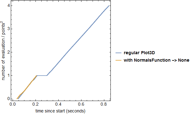
I also generated a timingNoNormals by adding NormalsFunction -> None to the above code, keeping everything else identical. Here are the results, presented graphically:

ListLinePlot[
  {timing, timingNoNormals},
  Frame -> True, Axes -> False, AspectRatio -> 1, FrameStyle -> Black,
  FrameLabel -> {"time since start (seconds)", "number of evaluation / points^2"},
  PlotLegends -> {"regular Plot3D", "with NormalsFunction -> None"}
]
comparison

Two features here were surprising to me, which lead to my questions:

  • I was surprised to find that a good 3/4 of the evaluation time in Plot3D seems to be taken up by calculation of the vertex normals. This can use up quite a bit of time for even moderately costly function. When can we safely turn this "feature" off using NormalsFunction -> None? Would it be safe to make that option persistent?

  • Additionally, the delay between the first batch of function evaluations and the second, corresponding to that plateau in the blue plot above, was surprising to me. What is Plot3D doing in between? Building a Graphics3D object?

$\endgroup$
1
  • 1
    $\begingroup$ It could be useful to additionally speed interactive cases up: NormalsFunction -> ControlActive[None, Automatic] $\endgroup$
    – Kuba
    Commented Jun 7, 2018 at 8:51

1 Answer 1

8
$\begingroup$

I observed that you included a timing before the plot, you missed a timing after the plot. Moreover, it appeared to me that TimeObject has quite an overhead, so in order to get "purer" timings, I replaced it by AbsoluteTime[]. This is what I used for timings:

points = 100;
f = {x, y} \[Function] x y;

opts = {PlotPoints -> points, MaxRecursion -> 0};
timing = Module[{i, start, results}, i = 0;
   results = Reap[
     Sow[{start = AbsoluteTime[], i++/points^2}];
     p = Plot3D[f[x,y], {x, -2, 2}, {y, -2, 2},
       Evaluate[opts],
       EvaluationMonitor :> Sow[{AbsoluteTime[], i++/points^2}]
       ];
     Sow[{AbsoluteTime[], i++/points^2}];
     ];
   {#1 - start, #2} & @@@ results[[2, 1]]];

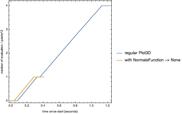
Then I got this

enter image description here

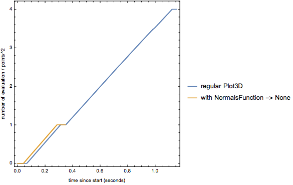
So it's not for sure that there is no plateau for the normal-free case. I'd say that a major part of the plateaus in the end are due to the mesh lines because they get shorter with Mesh -> None. These are the timings without the mesh lines:

enter image description here

Moreover, there is some time needed to compute the polygon index lists for the final GraphicsComplex. This won't need any point evaluations (the points are already evaluated), so this will also contribute the the plateaus.

Notice also the small shift between the yellow and the first blue ramp. This could be the infamous 50 ms that might be due to compilation of the normal function into "WVM".

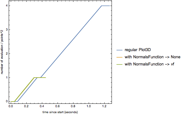
In the end, I still wonder what Mathematica is doing with the normal. In particular because you can get rid virtually all the time spent for "computing the vertex normals" by specifying your own NormalFunction like this:

νf = {x, y} \[Function] Evaluate[Cross @@ Transpose[D[{x, y, f[x, y]}, {{x, y}, 1}]]];
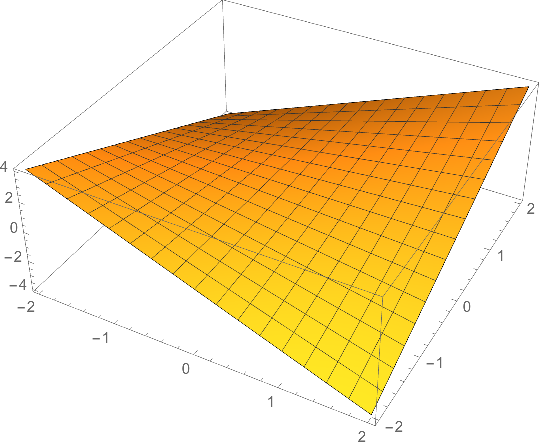
Plot3D[f[x, y], {x, -2, 2}, {y, -2, 2},NormalsFunction -> νf, Evaluate[opts]]

enter image description here

If the function f is sufficiently smooth, this will result in a perfect plot and the following timings

enter image description here

Addendum

If I needed many plots quickly, I would do the following:

points = 100;
mesh = {15, 15};
f = {x, y} \[Function] x y;
νf = {x, y} \[Function] Evaluate[-Cross @@ Transpose[D[{x, y, f[x, y]}, {{x, y}, 1}]]];

cfsurface = 
  With[{code = {Compile`GetElement[X, 1], Compile`GetElement[X, 2], 
      f[Compile`GetElement[X, 1], Compile`GetElement[X, 2]]}},
   Compile[{{X, _Real, 1}}, code, RuntimeAttributes -> {Listable}, Parallelization -> True]
   ];
cνf = 
  With[{code = νf[Compile`GetElement[X, 1], Compile`GetElement[X, 2]]},
   Compile[{{X, _Real, 1}}, code, RuntimeAttributes -> {Listable}, 
    Parallelization -> True]
   ];
getQuads = Compile[{{m, _Integer}, {n, _Integer}},
   Flatten[Table[
     {m (j - 1) + i, m (j - 1) + i + 1, m j + i + 1, m j + i},
     {j, 1, n - 1}, {i, 1, m - 1}], 1],
   CompilationTarget -> "C",
   RuntimeOptions -> "Speed"
   ];

points = 100;
pts2D = Tuples[{Subdivide[-2., 2., points - 1], Subdivide[-2., 2., points - 1]}];
lines = cfsurface@Outer[List, Subdivide[-2., 2., mesh[[1]] - 1], Subdivide[-2., 2., mesh[[2]] - 1]];
Graphics3D[{
  GraphicsComplex[
   cfsurface[pts2D], {EdgeForm[], Orange, Specularity[White, 30], 
    Polygon[getQuads[points, points]]}, 
   VertexNormals -> c\[Nu]f[pts2D]],
  Line@lines,
  Line@Transpose[lines]
  },
 Lighting -> "Neutral"
 ]

Even with compilation time included, this takes just 0.1 seconds (and about 0.018 seconds without compilation time).

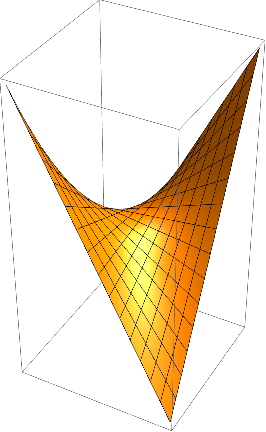
enter image description here

$\endgroup$
2
  • $\begingroup$ This is very nice, thank you! $\endgroup$
    – MarcoB
    Commented Jun 9, 2018 at 17:08
  • $\begingroup$ You're always welcome! $\endgroup$ Commented Jun 9, 2018 at 17:08

Your Answer

By clicking “Post Your Answer”, you agree to our terms of service and acknowledge you have read our privacy policy.

Not the answer you're looking for? Browse other questions tagged or ask your own question.