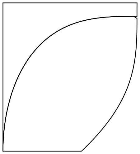
The "canonical" way is to find a pattern (here, {Black, Thick}) that matches what the boundary is made of and extract it from the graphics object.
So given
pt = RegionPlot[{{x^3 - y^2 > 2 y &&
     x^2 + y^3 > 2 x}, {x^3 - y^2 < 2 y && x^2 + y^3 > 2 x}}, {x, -1,
   1}, {y, -1, .1}, PlotStyle -> {Green, Yellow},
  BoundaryStyle -> {Black, Thick}];

bdy=Cases[Normal@First@pt, {Black, Thick, __}, Infinity];

Graphics[bdy]

---EDIT 2---
In diagonally reading your question, I missed the requirement for the boundary between the two.
The following will work on the particular dataset. First, you can extract the points from the bdy:
points = Cases[bdy, Line[a___] -> a, Infinity]
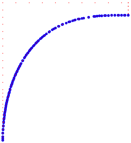
and you will notice that there are two components each corresponding to one region. Now a nearest function on one set of points applied to the second should give you their boundary:
With[{nf = Nearest[points[[2]]]},
 Show[Graphics[{Blue, PointSize -> Large,
    Point[Flatten[nf /@ points[[1]], 1]]}],
  Graphics[{Red, PointSize -> Small, Point[points[[2]]]}]]
 ]

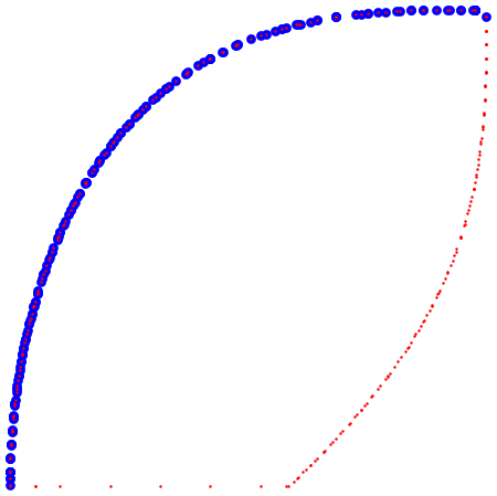
(and interchanging the components should yield more or less the same result)
With[{nf = Nearest[points[[1]]]},
 Show[Graphics[{Blue, PointSize -> Large,
    Point[Flatten[nf /@ points[[2]], 1]]}],
  Graphics[{Red, PointSize -> Small, Point[points[[1]]]}]]
 ]

so now you haveI thought that Intersection wouldn't work for the boundarytwo but as @eldo points to fit to a model of your liking or interpolate or whatever you wantout, it turns out it does:
With[{nf = Nearest[points[[2]]]},
 bdy = Flatten[nf /@ points[[2]], 1]];
 bdy = First /@ GatherBy[bdyGatherBy[Intersection@@points, First] (* so that there are no duplicate x coordscoords*);
 ]
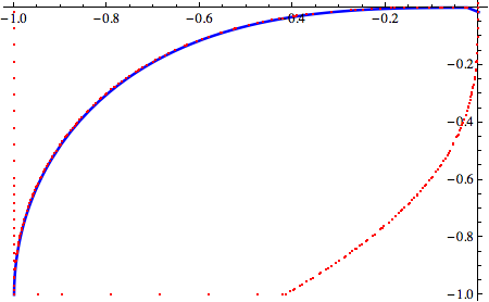
i.e.gives the boundary points which can be fitted to a model of your liking or interpolate or whatever:
 fit = Interpolation[bdy, InterpolationOrder -> 1];

Plot[fit[x], {x, -1, 0},
 Epilog -> {Red, PointSize -> Tiny, Point[points[[1]]~Join~points[[2]]]},
  PlotStyle -> {Blue, Thick}]

