On postprocessing and DisplayFunction
My thought, when the question was first posted, was to postprocess the
coordinates (see below), as is often done when graphics need to be transformed.
Before I was ready to post, @cvgmt posted their answer. At first I thought I'd
let it go, but metroidman's
reaction
made me think some clarification was needed, at least for other site visitors.
Aside from the (ab)use of DisplayFunction, the difficulties in getting a
good-looking plot by transforming coordinates, some of which are apparent in the
examples, have yet to be explained. Aside from these reasons for this post,
the really cool is buried down there where you probably won't even find it.
Whether we use Plot[] or ContourPlot[] or simply Graphics[],
there's no difference between the following three,
Plot[..., DisplayFunction -> f]
Show[Plot[...], DisplayFunction -> f]
Plot[...] // f
except that in the latter, the code is shorter and there is no mystery to anyone
reading the code how f is applied. Hence the most straightforward way is to
postprocess the graphics (I've usually done something similar to what @kglr does
in
Polar contour plot in Mathematica?
when I know the coordinates are stored in a GraphicsComplex):
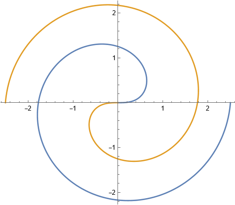
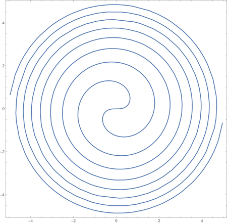
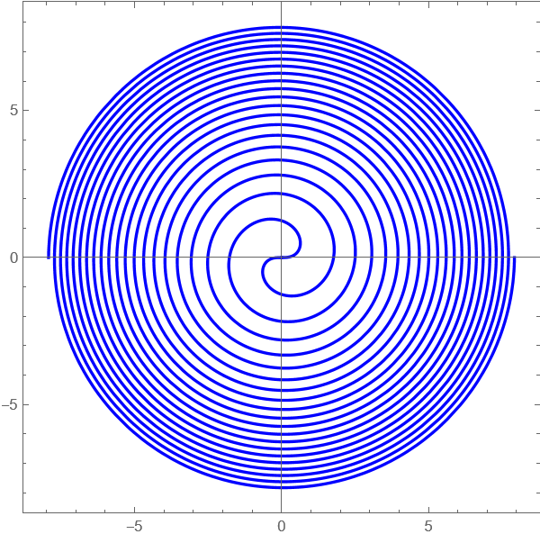
ContourPlot[r^2 == t
  , {t, 0, 8 Pi}, {r, -5, 5}
  , PlotPoints -> 4*15, MaxRecursion -> 3] /.
 Graphics[g_, opts___] :> Graphics[
   g /. GraphicsComplex[p_, rest__] :>
     GraphicsComplex[Function[{t, r}, r {Cos[t], Sin[t]}] @@@ p,
      rest]
   , PlotRange -> All (* needed *)
   , Ticks -> Automatic, FrameTicks -> Automatic, Axes -> True (* cosmetic *)
   , opts]
What problems do all the extra options address, if any?
Problems and solutions
1. Converting only coordinates.
This form keeps the coordinate conversion from being applied to non-coordinate
pairs of numbers (or triples in the case of 3D graphics). Some graphics forms
are difficult to transform, like Text[{0.7, 1.3}, {1.,0.83}, {0.,0.5}, {1.,1.}], but they rarely show up in straight plots. The best approach is to
make such annotations after coordinate conversion. This slight modification of
another answer fails, for instance, because the PlotRange is altered by the
DisplayFunction:
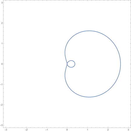
ContourPlot[r == (r - Cos[t])^2, {r, -3, 3}, {t, -3., 3.},
 DisplayFunction ->
  ReplaceAll[{r_Real, t_Real} :> {r*Cos[t], r*Sin[t]}],
 PlotPoints -> 80]
2. Getting a smooth polar plot.
The meshing and subdivision algorithms of the plotting function are based on
measures of lengths, areas, and angles in cartesian coordinates. When the
results are transformed, angles may be magnified and lengths and areas scaled.
The results may not look pretty. Hence we see larger settings than normal of
PlotPoints and MaxRecursion. It results in overkill for some regions of a
plot, but it's the most convenient way to get a smooth curve. Unfortunately
there is no way other than trial and error to determine what is a sufficiently
high setting. The setting for PlotPoints that I chose, 4*15, corresponds to
fifteen points per period, which is not a lot; so I bumped up MaxRecursion to
add more points where needed. In other examples in this Q&A, one sees PlotPoints -> 80
here and PlotPoints -> 100 there. These are rather high compared to the default
setting PlotPoints -> 15. Also, if I change the domain for the angle
t, then I will probably have to change the PlotPoints setting, a minor
annoyance.
3. Seeing the plot.
The plot range in cartesian coordinates and the plot range in polar coordinates
are not the same. If PlotRange is set in the cartesian graph being
transformed, it needs to be reset in the polar plot. PlotRange -> All is
convenient for showing all the plot, which can be seen in some examples in this Q&A.
Generally, you may have to figure out how
to zoom in on a certain portion if All is not what you want to show.
Historical notes on DisplayFunction
The intended use of DisplayFunction is to display the graphics, which as
@goofy
notes
was not originally automatic
(see Basic questions about running Mathematica, for instance).
It was used to control whether the graphics were
to be displayed at all or to send the PostScript form of the graphics to another
stream. In V6 Display[] became obsolete
(see What does DisplayFunction->Identity do to graphics functions?),
and the purpose of applying
DisplayFunction to graphics changed in the docs from "in order to display them" to "before
returning them." The examples still show different ways to display graphics,
and an example can be found in
How to set the output be generated in a cell different from "Output".
Nowadays, it has been repurposed by the "Marketing" plot theme to add elements
to 3D plots; its usefulness is shown in
How to get a black transparent background in Plot3D?
In this way a plot theme would not conflict with a user-specified Epilog; however,
there would be a conflict with a user-specified DisplayFunction. A user might
be better off using Epilog to get the background effects of "Marketing".
A look at the evolving documentation
From V1:
DisplayFunction is an option for graphics functions that specifies the
function to apply to the graphics primitives that are generated in order to
display them. The default setting for DisplayFunction is
$DisplayFunction. A typical setting is
DisplayFunction->Display[channel, #]&. Setting
DisplayFunction->Identity will cause graphics primitives to be
returned, but no display to be generated.
V2 added sound and a DisplayFunction for sound objects; otherwise, the
documentation and intended use didn't change until V6. In V6, the default
setting for $DisplayFunction became Identity and Graphics and Graphics3D
output were automatically rendered. Another change in V6:
Show, as well as functions like Plot and Plot3D, automatically apply the
function specified by the setting for DisplayFunction before returning their
results.
Prior to that, if graphics were returned, they were typeset as (literally) -Graphics-
or -SurfaceGraphics- etc.
Polar contour plots
Code for polarEquationPlot[] may be found on Github or in the code dump below.
The function uses the FEM functionality to make a mesh that resolves the features
of the curve. It adds a few MaxCellMeasure options:
{ (* override with MaxCellMeasure->opts *)
 "Area" -> 10. (* refine if (polar) area greater *)
 , "Length" -> 0.65 (* refine if r*dt greater *)
 , "Angle" -> 0.25 (* refine if dt greater *)
 , "Curvature" -> 0.5 (* refine if curvature greater *)
 , "MinArea" -> 0.0005 (* stop mesh refinement *)
 }
Curvature estimation is numerical and not very good until the mesh is small.
Graphics options, some ToElementMesh[] options, and some plotting options should work.
Works on my examples; hope it works on yours; otherwise, I'll delete.
Not much in the way of error checking yet.
Load package (maybe someday I'll have time to put together a paclet for the WPR):
Get["https://raw.githubusercontent.com/mroge02/polarEquationPlot/main/polarEquationPlot.wl"]
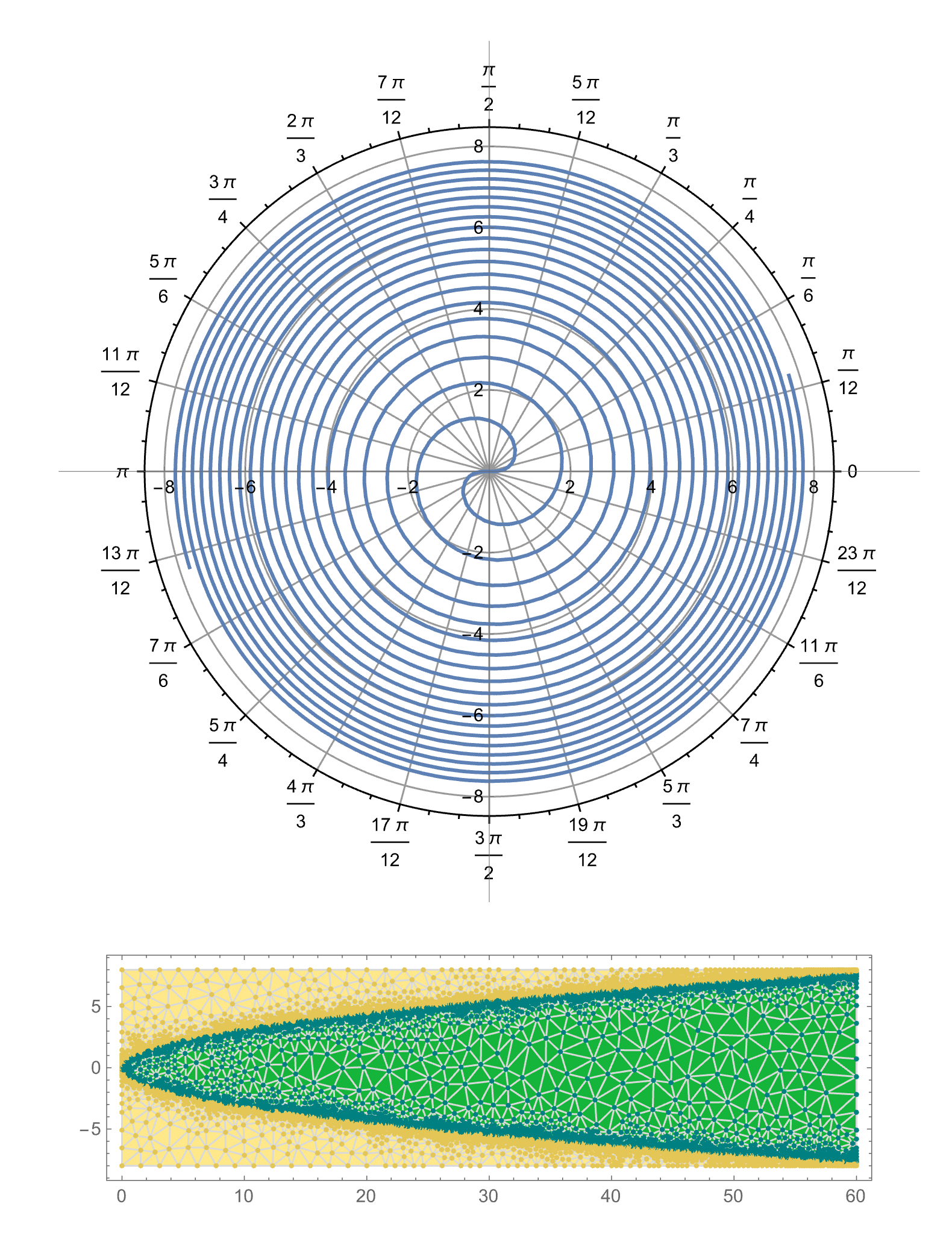
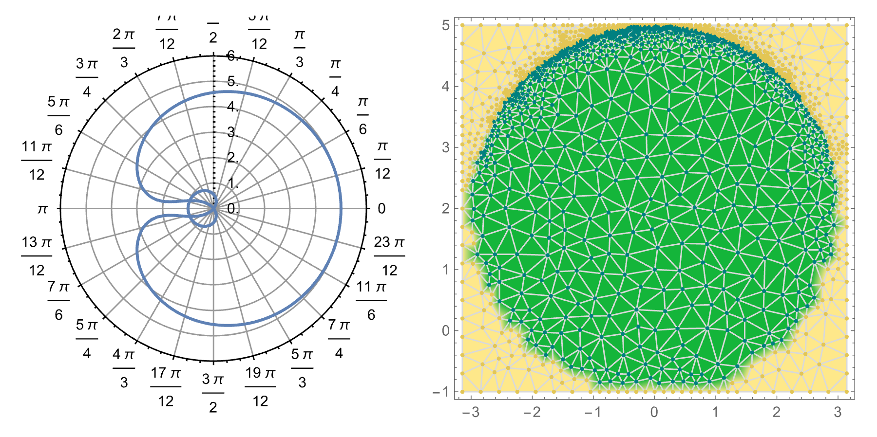
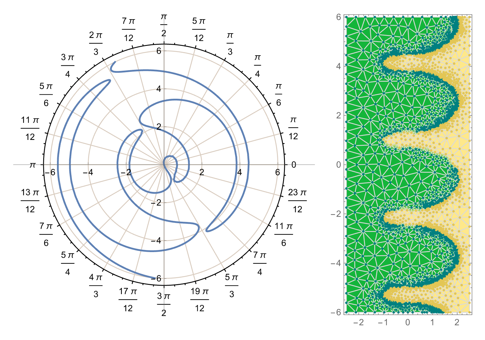
Examples show both the generated plot and the mesh that was computed to create the plot.
GraphicsColumn[{
  polarEquationPlot[r^2 == t, {t, 0, 60}, {r, -8, 8},
   PolarAxes -> Automatic, Axes -> True, PolarGridLines -> Automatic,
   ImageSize -> Large],
  getLastPolarMeshPlot[]
  }]

GraphicsRow[{
  polarEquationPlot[(r - 2)^2 + t^2 == 9, {t, -Pi, Pi}, {r, -1, 5},
   PolarAxes -> True, PolarGridLines -> Automatic],
  getLastPolarMeshPlot[]
  }]

GraphicsRow[{
 (* poor curvature refinement *)
 polarEquationPlot[
  10 Cos[(r - 1)]^2 + t^3 == 9, {t, -2.5, 2.5}, {r, -6, 6},
  MaxCellMeasure -> {"Curvature" -> 0.05}, PolarAxes -> Automatic,
  Axes -> True, PolarGridLines -> Automatic,
  GridLinesStyle -> RGBColor[0.85, 0.8, 0.75]],
 getLastPolarMeshPlot[]
 }]

Code dump
(* polarEquationPlot` Package v0.1 \[LongDash] ToElementMesh[] *)

BeginPackage["polarEquationPlot`"];

polarEquationPlot // ClearAll; (* Main function *)
lastPolarEquationPlotData // ClearAll; (* plot data (for debugging) *)
getLastPolarMeshPlot // ClearAll; (* visualizes last mesh (for debugging) *)


Begin["`Private`"];

Needs["NDSolve`FEM`"];

(*"
 * Main Function
"*)

polarEquationPlot // Options = Join[
   {MaxCellMeasure -> Automatic},
   Normal@KeyDrop[Options@PolarPlot, {MaxRecursion, PlotPoints}]];
call : polarEquationPlot[f_, {t_, t1_, t2_}, {r_, r1_, r2_},
   opts : OptionsPattern[]] :=
 With[{data = createPlotData @@ Unevaluated[call]},
  iPolarEquationPlot[data] /; FreeQ[data, Failure | createPlotData]
  ]

(* TBD *)
$unimplementedOptions = {ColorFunction, ColorFunctionScaling,
   EvaluationMonitor, Exclusions, ExclusionsStyle, LabelingSize, Mesh,
   MeshFunctions, MeshShading, MeshStyle, PerformanceGoal, PlotLabels,
   PlotLegends, PlotStyle, PlotTheme, RegionFunction, ScalingFunctions,
   WorkingPrecision};

(*"
 * Utilities
 *   createPlotData - process arguments and make plotData structure
 *   polarCurvature - estimate curvature of f[r, t] == 0
 *   meshRefine - refine mesh by measuring size/curvature in polar space
 *   makePolarGrid - steal polar grid from ListPolarPlot
 *   toLine - convert an intersected triangle into a crossing line
 *   toPoint - convert a crossed edge into a point of intersection
"*)

polarCurvature // ClearAll;
polarCurvature[points_, fvalues_, r1_ : Automatic] :=
  Module[{r0, derivs, denom},
   r0 = Replace[r1, Automatic :> Abs@Mean[points[[All, 2]]]];
   (* quadratic appoximation *)
   derivs =
    LeastSquares[Function[{t, r}, {1., t, r, t^2/2, r t, r^2/2}] @@@ points,
     fvalues];
   denom = r0^2 derivs[[2]]^2 + derivs[[3]]^2;
   If[denom == 0,(* rare *)
    100.,(* arbitrary large curvature *)
    (r0^2 derivs[[2]]^3 - 2 derivs[[2]]^2 derivs[[3]] +
        r0 derivs[[3]]^2 derivs[[4]] -
        2 r0 derivs[[2]] derivs[[3]] derivs[[5]] +
        r0 derivs[[2]]^2 derivs[[6]])/(denom)^(3/2) // Abs
    ]
   ];
(*"
 * meshRefine[] is used in iPolarEquationPlot[] to control refinement of mesh
 *    Parameters are defined by options processed by createPlotData[]
"*)
meshRefine // ClearAll;
(* parameters may be set by polarEquationPlot[] *)
$plotData = <|
   (* override with MaxCellMeasure->opts *)
   "Area" -> 10. (* refine if (polar) area greater *)
   , "Length" -> 0.65 (* refine if r*dt greater *)
   , "Angle" -> 0.25 (* refine if dt greater *)
   , "Curvature" -> 0.5 (* refine if curvature greater *)
   , "MinArea" -> 0.0005 (* stop mesh refinement *)
   |>;
meshRefine[f_][vertices_, area_] := Module[{midpoints, pts, vals, r0, dt},
   r0 = Abs@Mean[vertices[[All, 2]]];
   If[r0*area > $plotData["Area"],
    True,
    If[(0.9 + r0) area > $plotData["MinArea"] &&
      Abs@Total@Sign[f @@@ vertices] < 3,
     dt = Max[vertices[[All, 1]]] - Min[vertices[[All, 1]]];
     If[dt > $plotData["Angle"] || r0*dt > $plotData["Length"],
      True,
      midpoints = Mean /@ Partition[vertices, 2, 1, 1];
      pts = Join[vertices, midpoints];
      vals = f @@@ pts;
      polarCurvature[pts, vals, r0] r0*dt > $plotData["Curvature"]
      ],
     False]]
   ];
createPlotData // Options = Options@polarEquationPlot;
createPlotData[f_, {t_, t1_, t2_}, {r_, r1_, r2_}, opts : OptionsPattern[]] :=
   Module[{plotData = $plotData, F, maxCellValue},
   With[{ff = f /. Equal -> Subtract},
    F = Replace[Hold[t, r],
      {Hold[tt_, rr_] :> (Block[{tt = #1, rr = #2}, ff] &),
       Hold[tt_[_], rr_[_]] :> (Block[{tt, rr}, t = #1; r = #2; ff] &)
       }]
    ];
   If[! NumericQ@F[t1, t2],
    (* MESSAGE *)
    Return[Failure["InvalidFunction",  <|
       "MessageTemplate" ->
        "Equation `Equation` did not evaluate to numeric values.",
       "MessageParameters" -> <|"Equation" -> f|>
       |>],
     Module],
    plotData["F"] = F
    ];
   If[! AllTrue[{t1, t2, r1, r2}, NumericQ],
    (* MESSAGE *)
    Return[
     Failure["InvalidDomain",  <|
       "MessageTemplate" -> "At least one of `Domain` is not numeric.",
       "MessageParameters" -> <|"Domain" -> {t1, t2, r1, r2}|>
       |>],
     Module],
    plotData["R"] = {r1, r2};
    plotData["T"] = {t1, t2}
    ];
   maxCellValue = OptionValue[MaxCellMeasure];
   If[NumericQ[maxCellValue],
    plotData["Area"] = maxCellValue,
    Switch[maxCellValue,
     {___Rule}
     , plotData = Merge[{plotData, maxCellValue}, Last]
     ; If[! VectorQ[Keys[$plotData] /. plotData, Positive],
      (* MESSAGE *)
      Return[
       Failure["InvalidMaxCell",  <|
         "MessageTemplate" ->
          "Maxima cell bounds in `CellBounds` should be positive real \
numbers.",
         "MessageParameters" -> <|"CellBounds" -> OptionValue[MaxCellMeasure]|>
         |>],
       Module]],
     Automatic
     , Null,
     _
     ,(* MESSAGE *)
     Null (* ignore??? *)
     ]
    ];
   plotData["GraphicsOptions"] =
    FilterRules[Flatten@{opts}, Options@PolarPlot];
   plotData
   ];
(*" Convert triangle to contour line
 *    Different signs => contour crosses edge
 *    Sign all equal => no contour line
 *    One vertex zero => contour line thru opp. edge if signs !=
 *    Two vertex zeros => contour line = edge
 *    Three vertex zeros => contour lines = all edges
"*)
toLine // ClearAll;
(*toLine[signs_,sum_,zeros_,idcs_]:= line;*)
toLine[signs_, sum_, 3, idcs_] :=
  Partition[Transpose[{idcs, idcs}], 2, 1, 1]; (* what to do? *)
toLine[signs_, 3 | -3, zeros_, idcs_] := {}; (* no crossings *)
toLine[signs_, sum_, 2,
   idcs_] := {{#, #} & /@ Extract[idcs, Position[signs, 0]]};
toLine[signs_, 2 | -2, 1, idcs_] := {};
toLine[signs_, 0, 1,
   idcs_] := {{{#, #} &@First@Extract[idcs, Position[signs, 0]],
    Extract[idcs, Position[signs, Except[0, _Integer]]]}};
toLine[signs_, 1, 0,
   idcs_] := {Transpose@{{#, #} &@First@Extract[idcs, Position[signs, -1]],
     Extract[idcs, Position[signs, 1]]}};
toLine[signs_, -1, 0,
   idcs_] := {Transpose@{{#, #} &@First@Extract[idcs, Position[signs, 1]],
     Extract[idcs, Position[signs, -1]]}};
(*"
 * Get crossing point from edge=idcs
"*)
toPoint // ClearAll;
toPoint[coords_, vals_, {i_, i_}] := coords[[i]];
toPoint[coords_, vals_, idcs_] := Cross[vals[[idcs]]] . coords[[idcs]]/
  Subtract @@ vals[[idcs]];
(*"
 * Get polar grid from ListPolarPlot
"*)
makePolarGrid // ClearAll;
makePolarGrid // Options =
  FilterRules[
   Options@PolarPlot, {PolarAxes, PolarGridLines, GridLinesStyle,
    PolarAxesOrigin}](*{PolarAxes\[Rule]Automatic,PolarGridLines\[Rule]\
Automatic,GridLinesStyle->Automatic,PolarAxesOrigin->Automatic}*);
makePolarGrid[0 | 0., OptionsPattern[]] := {};
makePolarGrid[r_?NumericQ, OptionsPattern[]] := First@DeleteCases[
    ListPolarPlot[{{0, r}}
     , PolarAxes -> OptionValue[PolarAxes]
     , PolarAxesOrigin -> OptionValue[PolarAxesOrigin]
     , PolarGridLines -> Replace[OptionValue[PolarGridLines]
       , {Automatic :> {Automatic, FindDivisions[{0, r}, 6]}
        , {theta_, Automatic} :> {theta, FindDivisions[{0, r}, 6]}}]
     , GridLinesStyle -> OptionValue[GridLinesStyle]
     , PlotRange -> All
     ]
    , _GraphicsComplex, Infinity];
(*"
 * Visualization of underlying mesh
"*)
getLastPolarMeshPlot // ClearAll;
getLastPolarMeshPlot // Options = Options@Graphics;
With[{
   polyStyles = {RGBColor[
     0.07843150501697072, 0.7098038624759535, 0.22745093193374122`, 1.],
     RGBColor[0.9941176941165422, 0.9098039188905757, 0.5431372307229443, 1.],
      RGBColor[
     0.8078430800811591, 0.06666710941434106, 0.1490195899430818,
      1.]}(*CountryData["Mali","Flag"]//DominantColors//MapAt[Lighter[#,
   0.5]&,#,2]&*),
   ptStyles = {Darker[Cyan, 0.5], Lighter@Blend[{Yellow, Darker@Orange}]}
   },
  getLastPolarMeshPlot[opts : OptionsPattern[]] := With[{
     mesh = lastPolarEquationPlotData["Mesh"],
     vals = 1 + UnitStep@lastPolarEquationPlotData["ValuesOnGrid"]},
    Graphics[
     MapAt[
      Append[#, {FaceForm[], (mesh@
            "Wireframe"["MeshElementStyle" -> EdgeForm@LightGray])[[1, 2, 2]],
          Point[Range@Length@vals, VertexColors -> ptStyles[[vals]]]
         }
        ] &,
      ElementMeshToGraphicsComplex[mesh, VertexColors -> polyStyles[[vals]]],
      2],
     opts,
     Frame -> True
     ]
    ]
  ];

(*"
 * Internal plotter
"*)

iPolarEquationPlot // ClearAll;
$gridPadding = Scaled[0.06];
iPolarEquationPlot[data_] := Block[{$plotData = data},
   Module[{coords,(*vals,*)signs, crossed, lines},
    glurg = foo = {};
    lastPolarEquationPlotData = data;
    lastPolarEquationPlotData["Mesh"] = ToElementMesh[
      Rectangle @@ Transpose@{data["T"], data["R"]},
      "MeshRefinementFunction" -> meshRefine[data["F"]],
      "MeshOrder" -> 1
      ];
    coords = lastPolarEquationPlotData["Mesh"]@"Coordinates";
    lastPolarEquationPlotData["ValuesOnGrid"] = data["F"] @@ Transpose[coords];
    signs =
     Sign[Threshold[lastPolarEquationPlotData["ValuesOnGrid"](*,
       AccuracyGoal?*)]];
    crossed =
     Pick[lastPolarEquationPlotData["Mesh"]["MeshElements"][[1, 1]],
      Abs@Total[signs[[#]]] < 3 & /@
       lastPolarEquationPlotData["Mesh"]["MeshElements"][[1, 1]]];
    murf = lines = Apply[Join,
       With[{s = signs[[#]]},
          With[{res = toLine[s, Total[s], Count[s, 0], #]},
           (*If[(*Count[res,{{x_,x_},{y_,y_}},Infinity]>1*)ArrayDepth[res]!=
           3,
           foo={foo,Inactive[toLine][s,Total[s],Count[s,0],#]}]*)
           foo = {foo, Inactive[toLine][s, Total[s], Count[s, 0], #]};
           res
           ]
          ] & /@ crossed
       ];
    With[{pr = Max@Abs[lastPolarEquationPlotData["Mesh"]@"Bounds" // Last]},
     Graphics[{
       makePolarGrid[
        Replace[$gridPadding, {Scaled[relPad_] :> (1 + relPad) pr,
          absPad_?NumericQ :> pr + absPad}],
        FilterRules[lastPolarEquationPlotData["GraphicsOptions"],
         Options@makePolarGrid]],
       "DefaultPlotStyle" /. (Method /.
           Charting`ResolvePlotTheme[Automatic, ContourPlot]) // First,
       Line[#[[2]] {Cos[#[[1]]], Sin[#[[1]]]} &@Block[{res},
              Check[

               res = toPoint[coords,
                 lastPolarEquationPlotData["ValuesOnGrid"], #],
               Echo[Length@Flatten@glurg + 1];
               ];
              glurg = {glurg, Hold[toPoint[
                  lastPolarEquationPlotData["Mesh"]@"Coordinates",
                  lastPolarEquationPlotData["ValuesOnGrid"],
                  #]]};
              res
              ] & /@ #] & /@ lines
       }
      , lastPolarEquationPlotData["GraphicsOptions"]
      , PlotRange -> All,
      PlotRangePadding ->
       If[MatchQ[PolarAxes /. lastPolarEquationPlotData["GraphicsOptions"],
         True | Automatic], Scaled[.1], Automatic]
      , Frame -> False
      , Axes -> !
        MatchQ[PolarAxes /. lastPolarEquationPlotData["GraphicsOptions"],
         True | Automatic]
      , Ticks -> ({#, #} &@
         Select[FindDivisions[{-pr, pr}, 8], -pr <= # <= pr &])
      ]
     ]]];

End[];

EndPackage[];

