3
$\begingroup$

I know this error is very common. I checked out a good number of proposed solutions to this problem, but unfortunately, none of them helped in my case.

I would appreciate any help or hints on how to overcome this issue.

My program is quite simple. It is supposed to solve two coupled time-dependent partial differential equations on a sphere. I don't know if it's relevant, but from the physical point of view, it's actually the semi-classical approximation of a modified Schrodinger's equation on a sphere, with the Newtonian gravitational potential made scale-invariant.

The program is supposed to solve the PDE up to t=100, but it breaks down even at a value as low as 0.01. Here's the code with some comments for further information:

  (* defining the potential that will be used in the equations. *)

V[ϕ_, θ_] := 
  0.045360921162651446/Sqrt[1 + Cos[ϕ] Sin[θ]] + 
   0.045360921162651446/Sqrt[
   1 - Sin[θ] Sin[π/6 - ϕ]] + 0.045360921162651446/
   Sqrt[1 - Sin[θ] Sin[π/6 + ϕ]];

(* defining the region in which the differential equation is to be solved. θ = π/2 is avoided on purpose because of the singularities of V *)

Π1 = 
  ImplicitRegion[
   0 <= ϕ <= 2 π && 
    0 <= θ <= π/2 - 0.001, {ϕ, θ}];
Π2 = 
  ImplicitRegion[
   0 <= ϕ <= 
     2 π && π/2 + 
      0.001 <= θ <= π, {ϕ, θ}];
Π = RegionUnion[Π1, Π2];


(* defining the two coupled PDEs. *)

firsteq = {-D[Subscript[S, 0][ϕ, θ, t], t] == -V[ϕ, θ] + (Derivative[0, 1, 0][Subscript[S, 0]][ϕ, θ, t]^2 + 
       Sec[θ]^2*Derivative[1, 0, 0][Subscript[S, 0]][ϕ, θ, t]^2)}; 
secondeq = {-D[Subscript[S, 1][ϕ, θ, t], t] == -((-Tan[θ])*Derivative[0, 1, 0][Subscript[S, 0]][ϕ, θ, t] + 
        Derivative[0, 2, 0][Subscript[S, 0]][ϕ, θ, t] + Sec[θ]^2*Derivative[2, 0, 0][Subscript[S, 0]][ϕ, θ, t]) + 
      2*(Derivative[0, 1, 0][Subscript[S, 0]][ϕ, θ, t]*Derivative[0, 1, 0][Subscript[S, 1]][ϕ, θ, t] + 
        Sec[θ]^2*Derivative[1, 0, 0][Subscript[S, 0]][ϕ, θ, t]*Derivative[1, 0, 0][Subscript[S, 1]][ϕ, θ, t])}; 


(* defining the initial conditions *)

initial = {Subscript[S, 0][ϕ, θ, 0] == Sin[θ], 
   Subscript[S, 1][ϕ, θ, 0] == Sin[θ]^2};


Equations = Join[firsteq, secondeq, initial];


(* Solving the equations ... *)

Solution = 
  NDSolve[Equations, {Subscript[S, 0], Subscript[S, 1]}, {t, 0, 
    100}, {ϕ, θ} ∈ Π, 
   Method -> "Automatic"];

I get the error:

NDSolve::ndsz: At t == 0.011684614824200409`, step size is effectively zero; singularity or stiff system suspected.

The system is indeed singular. I plotted the incomplete solution and it appears that very soon the solution diverges over some regions near the poles and equator. Is there some way to overcome this problem?

Thank you very much.

Edit:

I modified the potential to remove its singularities:

V[ϕ_, θ_] := 
      0.045360921162651446/Sqrt[1.00001 + Cos[ϕ] Sin[θ]] + 
       0.045360921162651446/Sqrt[
       1.00001 - Sin[θ] Sin[π/6 - ϕ]] + 0.045360921162651446/
       Sqrt[1.00001 - Sin[θ] Sin[π/6 + ϕ]];

Following the suggestions in the comments, I tried to correct another issue in the code and define periodic boundary conditions for ϕ. Here's the code I added. I'm grateful to @xzczd for this.

  δ = 10^-5;
periodicity = {PeriodicBoundaryCondition[
    Subscript[S, 0][ϕ, θ, t], ϕ == 0 && 
     0 <= θ <= π , Function[x, x + {2 π, 0}]], 
   PeriodicBoundaryCondition[
    Subscript[S, 0][ϕ, θ, 
     t], ϕ == 2 π + δ && 0 <= θ <= π , 
    Function[x, x + {-2 π, 0}]], 
   PeriodicBoundaryCondition[
    Subscript[S, 1][ϕ, θ, t], ϕ == 0 && 
     0 <= θ <= π , Function[x, x + {2 π, 0}]], 
   PeriodicBoundaryCondition[
    Subscript[S, 1][ϕ, θ, 
     t], ϕ == 2 π + δ && 0 <= θ <= π , 
    Function[x, x + {-2 π, 0}]]};

But this time, I got this error:

NDSolve::ndcf: Repeated convergence test failure at t == 0.`; unable to continue.

Following @xzczd's helpful suggestion, I decided to forget about FiniteElements and use the TensorProduct method instead. Here's the final code. I also changed the initial conditions.

    firsteq = {-D[Subscript[S, 0][ϕ, θ, t], t] == -V[ϕ, θ] + (Derivative[0, 1, 0][Subscript[S, 0]][ϕ, θ, t]^2 + Csc[θ]^2*Derivative[1, 0, 0][Subscript[S, 0]][ϕ, θ, t]^2)}; 
    secondeq = {-D[Subscript[S, 1][ϕ, θ, t], t] == -((-Cot[θ])*Derivative[0, 1, 0][Subscript[S, 0]][ϕ, θ, t] + Derivative[0, 2, 0][Subscript[S, 0]][ϕ, θ, t] + Csc[θ]^2*Derivative[2, 0, 0][Subscript[S, 0]][ϕ, θ, t]) + 
          2*(Derivative[0, 1, 0][Subscript[S, 0]][ϕ, θ, t]*Derivative[0, 1, 0][Subscript[S, 1]][ϕ, θ, t] + Csc[θ]^2*Derivative[1, 0, 0][Subscript[S, 0]][ϕ, θ, t]*Derivative[1, 0, 0][Subscript[S, 1]][ϕ, θ, t])}; 
    
    
    initial = {Subscript[S, 0][ϕ, θ, 0] == Sin[θ]^2, 
               Subscript[S, 1][ϕ, θ, 0] == Sin[θ]^2};
        

Periodicity = {Subscript[S, 0][0, θ, t] == 
    Subscript[S, 0][2 π, θ, t], 
   Subscript[S, 1][0, θ, t] == 
    Subscript[S, 1][2 π, θ, t]};


            Equations = Join[firsteq, secondeq, initial, periodicity];
        
            Solution = 
                  NDSolve[Equations, {Subscript[S, 0], Subscript[S, 1]}, {t, 0, 
                    10}, {ϕ, 0, 2 π}, {θ, 0, π}, 
                   Method -> {"PDEDiscretization" -> {"MethodOfLines", 
                       "SpatialDiscretization" -> {"TensorProductGrid", 
                         "MaxPoints" -> 500, "MinPoints" -> 500}}}];

However, after about half an hour, I got this error:

NDSolve::ndsz: At t == 0.00003716693557750961`, step size is effectively zero; singularity or stiff system suspected.

NDSolve::eerr: Warning: scaled local spatial error estimate of 1.0182820651808292`*^12 at t = 0.00003716693557750961` in the direction of independent variable ϕ is much greater than the prescribed error tolerance. Grid spacing with 500 points may be too large to achieve the desired accuracy or precision. A singularity may have formed or a smaller grid spacing can be specified using the MaxStepSize or MinPoints method options.

I tried to make the discretization finer, but the kernel crashed for MaxPoints, MinPoints = 1000.

$\endgroup$
22
  • 1
    $\begingroup$ Hello! There are several problems. You specify $0\leq\phi\leq 2\pi$ in the domain and surely are thinking that angle $\phi = 0$ and angle $\phi = 2\pi$ must be identified. No, for Mathematica \[Phi] is just another symbol. You seem to think that you get away with simply cutting out a $0.001$-neighborhood near some singularity. No, you are creating a new boundary. Also, spherical coordinates are themselves singular at the north and south poles. $\endgroup$
    – user293787
    Commented Jul 24, 2022 at 14:11
  • $\begingroup$ I do not want discourage you. With the search phrase "[differential-equations] spherical coordinates" here on Mathematics SE I found this and this and this and this. Perhaps you can find some interesting hints or ideas there. $\endgroup$
    – user293787
    Commented Jul 24, 2022 at 14:23
  • 1
    $\begingroup$ But the missing boundary condition in $\phi$ direction is indeed a problem. See e.g. this and this. Also, since the problem is defined in a regular domain, I'd say the old-good TensorProductGrid is a better choice, see e.g. discussions here and here. And, I believe you need to re-consider the definition of the potential, can you turn to a potential free of singularity? $\endgroup$
    – xzczd
    Commented Jul 24, 2022 at 14:42
  • 1
    $\begingroup$ Currently FEM is automatically chosen because you've used Element and PeriodicBoundaryCondition in your code. (See this post for more info. ) Anyway, if you want to use PeriodicBoundaryCondition: t should not be part of the domain, because FiniteElement method is only used for spatial discretization, something like PeriodicBoundaryCondition[ Subscript[S, 0][\[Phi], \[Theta], t], \[Phi] == 0 && 0 <= \[Theta] <= \[Pi], Function[x, x + {2 \[Pi], 0}]] (You need to modify the other 3 accordingly, of course) should work. $\endgroup$
    – xzczd
    Commented Jul 25, 2022 at 1:58
  • 1
    $\begingroup$ The Sec[θ] term is undoubtedly hard to handle. There might exist certain clever variable transformation that can avoid this singularity (an example is this post) but I can't think out one. Anyway, by adding a relatively large artificial viscosity term (μ=10^-1) and choosing a relatively coarse grid (100 points for each dimension) I obtain the following $S_0$ (firsteq only involves $S_0$, so I solve it separately): i.sstatic.net/EhS5J.png Is this solution expected? $\endgroup$
    – xzczd
    Commented Jul 25, 2022 at 16:05

1 Answer 1

5
$\begingroup$

First of all, I'd like to emphasize again that it's important to make sure the equation system itself is correct. Anyway, after the correction the system is less demanding, so let me post an answer.

The idea is simple: the system is nonlinear, derivative of $S_0$ in $\theta$ direction of firsteq is of 1st order, derivative of $S_1$ in $\theta$ direction of secondeq is of 1st order, the solution of the system seems to be stiff, so the experience obtained in e.g. this post may help. Let's try artificial viscosity.

After adding artificial viscosity, something related to the issue discussed in this post seems to show up, so I use pdetoode to discretize the system.

V[ϕ_, θ_] := 
  0.045360921162651446/Sqrt[1.00001 + Cos[ϕ] Sin[θ]] + 
   0.045360921162651446/Sqrt[1.00001 - Sin[θ] Sin[π/6 - ϕ]] + 
   0.045360921162651446/Sqrt[1.00001 - Sin[θ] Sin[π/6 + ϕ]];

Clear[points, grid, domain]
points@ϕ = points@θ = 200;
eps = 0(*Pi/10^2*);
domain@ϕ = {0, 2 Pi}; domain@θ = {eps, Pi - eps};
(grid@# = Array[# &, points@#, domain@#]) & /@ {ϕ, θ};

difforder = 2;
(* Definition of pdetoode isn't included in this post,
   please find it in the link above. *)
ptoofunc = 
  pdetoode[{Subscript[S, 0], Subscript[S, 1]}[ϕ, θ, t], t, 
   grid /@ {ϕ, θ}, difforder, {True, False}];
μ0 = 10^-2; μ1 = 10^-2;
Unevaluated[
   eq = {μ0 (D[Subscript[S, 0], {θ, 2}] + 
          D[Subscript[S, 0], {ϕ, 2}]) - 
       D[Subscript[S, 0], 
        t] == -V[ϕ, θ] + (D[Subscript[S, 0], θ]^2 + 
         Csc[θ]^2 D[Subscript[S, 0], ϕ]^2), μ1 (D[Subscript[S, 
           1], {θ, 2}] + D[Subscript[S, 1], {ϕ, 2}]) - 
       D[Subscript[S, 1], 
        t] == -(-Cot[θ] D[Subscript[S, 0], θ] + 
          D[Subscript[S, 0], {θ, 2}] + 
          Csc[θ]^2 D[Subscript[S, 0], {ϕ, 2}]) + 
       2 (D[Subscript[S, 0], θ] D[Subscript[S, 1], θ] + 
          Csc[θ]^2 D[Subscript[S, 0], ϕ] D[Subscript[S, 1], ϕ])};
   ic = {Subscript[S, 0] == Sin[θ]^2, Subscript[S, 1] == Sin[θ]^2} /. 
     t -> 0;
   bc = {D[Subscript[S, 0], θ] == 0, 
      D[Subscript[S, 1], θ] == 
       0} /. {{θ -> domain[θ][[1]]}, {θ -> 
        domain[θ][[-1]]}}] /. {Subscript[S, 0] -> 
    Subscript[S, 0][ϕ, θ, t], 
   Subscript[S, 1] -> Subscript[S, 1][ϕ, θ, t]};
del = #[[2 ;; -2]] &;
ode = Map[del, ptoofunc@eq, {2}] // Quiet;

odebc = ptoofunc@diffbc[t][bc];
odeic = ptoofunc@ic;

varlst = Outer[#@##2 &, {Subscript[S, 0], Subscript[S, 1]}, grid@ϕ, 
   grid@θ];

tend = 10; 

showStatus[status_]:=LinkWrite[$ParentLink,
  SetNotebookStatusLine[FrontEnd`EvaluationNotebook[],ToString[status]]];
clearStatus[]:=showStatus[""];
clearStatus[]
jianshi[t_]:=EvaluationMonitor:>showStatus["t = "<>ToString[CForm[t]]]
 sollst = NDSolveValue[{ode, odeic, odebc}, varlst, {t, 0, tend}, jianshi[t], 
   Method -> {"EquationSimplification" -> "MassMatrix"}(*,SolveDelayed->
   True*)]; // AbsoluteTiming
(* {1984.24, Null} *)

{sols0, sols1} = rebuild[#, grid /@ {ϕ, θ}, -1] & /@ sollst;

Remark

Adding PrecisionGoal -> 3, AccuracyGoal -> 3 to NDSolveValue will reduce the timing to about 277.04 seconds! But the beginning part of $S_1$ (for about $t<0.2$) changes. (Not widely different, but quite observable. ) Anyway, if the accuracy of transient behavior isn't important for you, consider adding these options.

The showStatus is from this post.

I've solved $S_0$ and $S_1$ all in one, but since firsteq only involves $S_0$ (and further trial suggests it's easier to solve than secondeq), you may consider solve firsteq first.

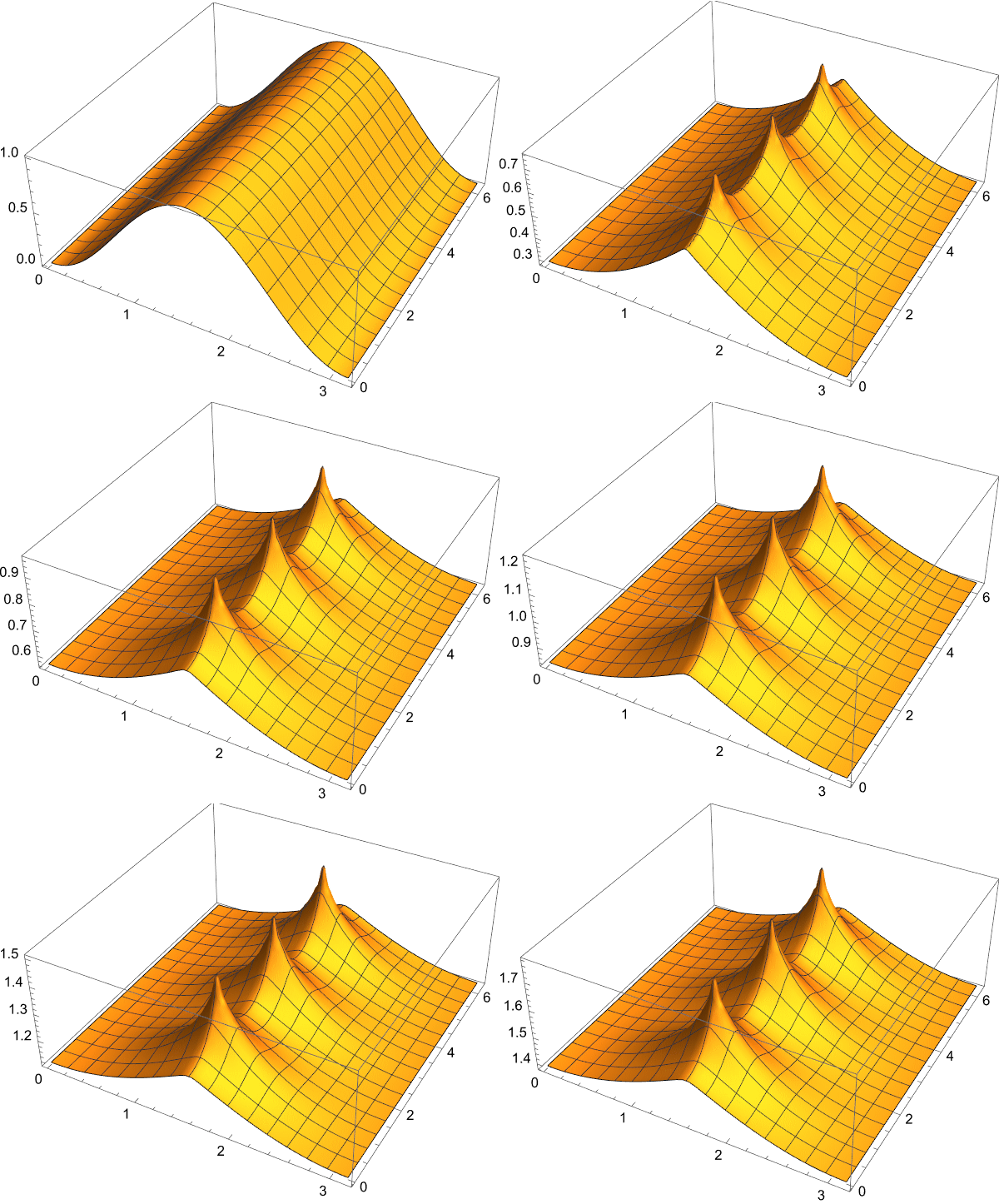
Let's check the solution. $S_0$:

piclst0 = Table[
   Plot3D[sols0[f, th, t], {th, #3, #4}, {f, #1, #2}, PlotPoints -> 50] & @@ 
    Flatten[domain /@ {ϕ, θ}], {t, 0, tend, tend/25}];

ListAnimate[piclst0]

enter image description here

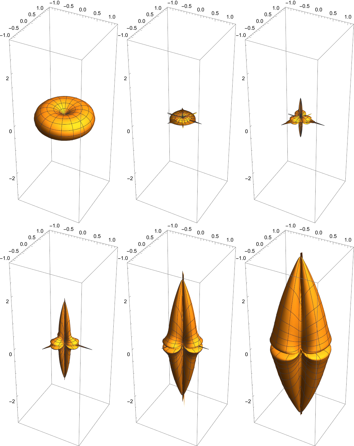
$S_1$:

piclst1 = Table[
   SphericalPlot3D[sols1[f, th, t], 
     {th, #3, #4}, {f, #1, #2}, PlotPoints -> 50] & @@
       Flatten[domain /@ {ϕ, θ}], {t, 0, tend, tend/25}];

ListAnimate[
 Show[#, PlotRange -> {{-1.2, 1.2}, {-1.2, 1.2}, {-3.2, 3.2}}] & /@ piclst1]

enter image description here

The solution around $\theta=\pi/2$ looks a bit unusual, I'm not sure if it's the nature of the solution or numeric error. You may adjust points@ϕ, points@θ, μ0, μ1 further to see how the solution changes.

$\endgroup$
5
  • $\begingroup$ It is a very nice solution (+1). Please note, first equation (the Hamilton-Jacobi equation) can be solved separately on Rectangle[{0,0}, {2 Pi, Pi}] without artificial viscosity. $\endgroup$ Commented Jul 26, 2022 at 10:10
  • $\begingroup$ @AlexTrounev Er… what setting do you choose? For points@ϕ = points@θ = 100;, NDSolve gets stuck around t==1.6 when solving firsteq; for points@ϕ = points@θ = 64; it gets stuck around t==2.6. (The steep potential function seems to be a problem. ) $\endgroup$
    – xzczd
    Commented Jul 26, 2022 at 13:14
  • $\begingroup$ Thank you very much for your answer. It helped a lot. I had been working on the program with your code. The viscosity term doesn't affect the dynamics very considerably but comes in handy especially for the first equation, as it tames the singular nodes that form. The only issue I face for some initial conditions is the computation time. Unless I run the code on a supercomputer or leave mine running for days (if not weeks!), the computation time can be an issue. Is there some way to increase the proficiency? $\endgroup$
    – Po_oya
    Commented Jul 30, 2022 at 20:08
  • $\begingroup$ I also tried to use this code for the full Schrodinger equation (without this approximation), but again faced the same error ("step size is effectively zero") which couldn't be solved by modifying the equations and adding the viscosity terms. Increasing the number of points was not a viable option either due to the huge computational load that would have been entailed. Anyway, that's a question I need to post separately. Thank you so much for your help. $\endgroup$
    – Po_oya
    Commented Jul 30, 2022 at 20:11
  • 1
    $\begingroup$ @Po_oya As to performance tuning, see the new-added Remark. $\endgroup$
    – xzczd
    Commented Jul 31, 2022 at 3:25

Your Answer

By clicking “Post Your Answer”, you agree to our terms of service and acknowledge you have read our privacy policy.

Not the answer you're looking for? Browse other questions tagged or ask your own question.