To help get you started I attempted to translate equation (5) from your snapshot into Mathematica.
Step 1
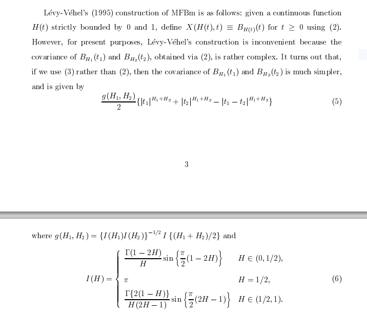
I(H) from the snapshot becomes:
i[h_] := Piecewise[{
   {Gamma[1 - 2 h]/h Sin[π/2 (1 - 2 h)], 0 < h < 1/2},
   {Gamma[2 (1 - h)]/(h (2 h - 1)) Sin[π/2 (2 h - 1)],
    1/2 < h < 1},
   {π, h == 1/2}
   }]
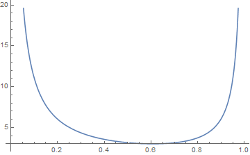
This is a function that can be plotted in the known range zero to one.
Plot[i[h], {h, 0, 1}]

Step 2
g(H1,H2) from the snapshot becomes:
g[h1_, h2_] := i[(h1 + h2)/2]/Sqrt[i[h1] i[h2]]
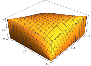
It can be plotted using the known range zero to one. Exclusions -> None was set so there are no interruptions where the derivative is discontinuous.
Plot3D[g[h1, h2], {h1, 0, 1}, {h2, 0, 1}, Exclusions -> None]

Step 3
In creating the covariance between BH1(t1) and BH2(t2) I will assume that t is greater than zero so the absolute times can be removed from all but the difference in time:
covB1B2[h1_, h2_, t1_, t2_] :=
 g[h1, h2]/2*(t1^(h1 + h2) + t2^(h1 + h2) - Abs[t1 - t2]^(h1 + h1))
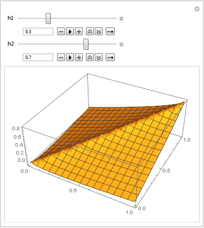
In order to plot this we need to make assumptions about the h1 and h2 values. Further we need to know the range of the time (I have no knowledge of this, nor do I know the time units). I chose zero to one for the time.
The function Manipulate can be used to dynamically set the h1 and h2 parameters.
Manipulate[
 Plot3D[covB1B2[h1, h2, t1, t2], {t1, 0, 1}, {t2, 0, 1},
  Exclusions -> None],
 {{h1, 0.3}, 0, 1, Appearance -> "Open"},
 {{h2, 0.7}, 0, 1, Appearance -> "Open"}
 ]

Change the parameters by using the slider or typing in the values.
