Why the BandpassFilter is different than applying LowpassFilter then HighpassFilter

Question

If I generate some data with noise, and use a filter to filter the noise, why does BandpassFilter not produce the same results as using LowpassFilter followed by HighpassFilter or vice-versa?

Here is the code:

data = Table[Sin[i^2 + i] + RandomReal[{-.2, .3}], {i, 0, Pi, 0.01}];

ListLinePlot /@ {data, 
  LowpassFilter[HighpassFilter[data, 0.01], 0.02], 
  HighpassFilter[LowpassFilter[data, 0.02], 0.01], 
  BandpassFilter[data, {0.01, 0.02}]}

Which produces plots like these:

It seems that either the high- plus low-pass or the low- plus high-pass filter combinations produce the same result, whereas the band pass filter produces a similar shape, but with a scaled $y$ value.

Why is that?

Answer 1

Original Answer

A good question to ask is: are these image processing filters or signal processing filters? If we take a signal processing viewpoint then it is useful to look at the impulse response function. First we make an impulse and then use your filters

imp = ConstantArray[0, 1024]; imp[[512]] = 1;
impR = {
     LowpassFilter[HighpassFilter[#, 0.01], 0.02],
     HighpassFilter[LowpassFilter[#, 0.02], 0.01],
     impR3 = BandpassFilter[#, {0.01, 0.02}]
     } &[imp];

 ListLinePlot[impR, PlotRange -> All, 
 PlotLegends -> LineLegend[{"HiLo", "LoHi", "Band"}]]

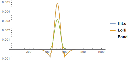
These are clearly smoothing filters with the High-Low the same as the Low-High. There are vertical steps in the output which I find strange. These are non-causal filters since they have output before the input arrives. From a signal processing viewpoint I don't work with non-causal filters but this may be normal in image processing. With a bit of rescaling they could be made to have the same central peak height but they would be different elsewhere. I also fail to see how the band pass filter is going to remove low frequencies since it has no negative part. To test this out I generate a constant value and filter

data2 = ConstantArray[1, 1024];
bp = BandpassFilter[data2, {0.01, 0.02}];
ListLinePlot[bp, PlotRange -> All]

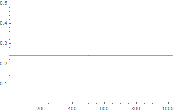
So the filter is not much good as a bandpass filter. Going farther we can look at the responses in the frequency domain.

 ft = Fourier[#, FourierParameters -> {-1, -1}] & /@ impR;
With[{n = 30},
 ListLinePlot[Evaluate[Abs[#[[1 ;; n]]] & /@ ft], PlotRange -> All, 
  PlotLegends -> LineLegend[{"HiLo", "LoHi", "Band"}], 
  DataRange -> {0, (n - 1) (2 \[Pi])/1024} ]]

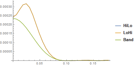
This spectra seems to agree that the bandpass filter is really a low pass filter. The high-low filters do seem to work. They seem a bit off with respect to the cutoff values specified. Overall I think these filters are for image processing. If you need filters for signal processing then look up ButterworthFilterModel or analogue filters. I would suggest, but am willing to be contradicted, that there is a muddle in the documentation between signal processing and image processing.

Your original question was why are the outputs different? If I was doing signal processing I could adjust my filters to give the same outputs by paying attention to filter orders and cut-off values. Without these details they would not be the same. I suspect that these filters are not designed to be equivalent.

Later thoughts

In the original question the bandwidth of the filter is very small and the filter center frequency is also small. This leads to the problem observed.

The definition of the frequency is important. In the above I have assumed a time step of 1. In general if the time step is dt then the sample rate sr is 1/dt. The time history may have frequency content between 0 and sr/2 as set by the Nyquist criterion. For simplicity actual frequencies are typically normalised by dividing by the sample rate thus the normalised frequency can run between 0 and 1/2. Further convenient normalisation includes a factor of 2 π so that the frequency content runs between between 0 and π. The frequencies used by BandpassFilter are expressed in this latter normalisation.

Thus the frequencies in the original question for the start and stop of the filter run between 0.01 and 0.02 this is a very small compared with the Nyquist frequency of 3.14159. Expressing this as center frequency and bandwidth the centre frequency is 0.015 and the bandwidth is 0.01.

The two functions that define a filter are the impulse response function and the frequency response function. The latter is the Fourier transform of the former. Here is the impulse response function for a bandpass filter that is just as narrow as the one in question but has a much larger center frequency.

ω = 1; (* center frquency *)
d = 0.1; (* bandwidth *)
nn = 100;(* number of points *)
irf = BandpassFilter[
   ArrayPad[{1}, nn/2], {ω - d/2, ω + d/2}];
ListLinePlot[irf, PlotRange -> All]

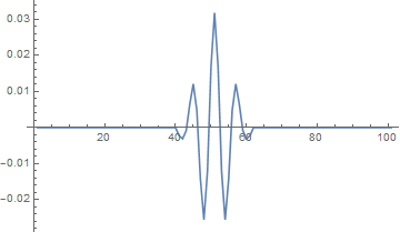
This looks fairly sensible. We take the Fourier transform to get the frequency response function.

frf = Abs@Fourier[irf, FourierParameters -> {-1, -1}];
ListLogPlot[
 Transpose[{Range[0, 2 π - (2 π)/(nn + 1), (2 π)/(
     nn + 1)], frf}][[1 ;; nn/2]], Joined -> True,
 Epilog -> {Pink, 
   Line[{{ω - d/2, Log@(10^-5)}, {ω - d/2, Log@1}}], 
   Line[{{ω + d/2, Log@(10^-5)}, {ω + d/2, Log@1}}]}, 
 Frame -> True, FrameLabel -> {"Frequency", "Spectral Amplitude"}, 
 ImageSize -> 8 72, PlotRange -> All]

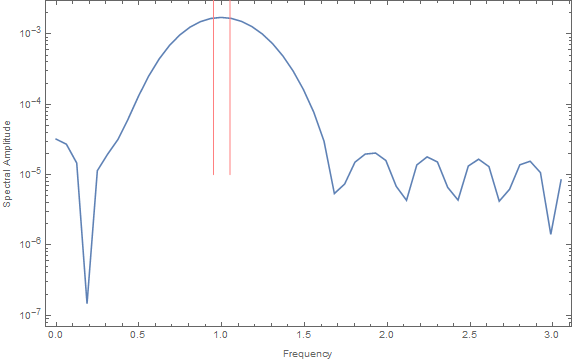
Again this is sensible with low and high frequencies being attenuated. We now look at a range of centre frequencies.

nn = 100; frfs = 
 Flatten[Table[
   Transpose[{Range[0, 2 π - (2 π)/(nn + 1), (2 π)/(
      nn + 1)], ConstantArray[ω, nn + 1], 
     Log@Abs@Fourier[
        BandpassFilter[
         ArrayPad[{1}, nn/2], {ω - 0.01, ω + 0.01}], 
        FourierParameters -> {-1, -1}]}], {ω, 0.02, π, 
    0.02}], 1]; ListPlot3D[frfs, PlotRange -> {{0, π}, All, All}, 
 AxesLabel -> {"Frequency", "Center Frequency", ""}, 
 ImageSize -> 8 72]

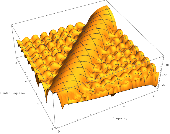
The band pass interval is the "half tube" that runs diagonally. The problem now becomes clear. At low center frequencies the "half tube" is missing on its low frequency side. Thus there is no low frequency effect. Thus for centre frequencies that are too small the band pass filter just behaves like a low pass filter.

I have made a dynamic that enables you to play with different centre frequencies and bandwidths.

DynamicModule[{nn = 100, d = 0.05, ω = π/2, spect, h},

 spect[ω_, d_, nn_] := 
  Abs@Fourier[
    BandpassFilter[
     ArrayPad[{1}, nn/2], {ω - d/2, ω + d/2}], 
    FourierParameters -> {-1, -1}];
 h = Transpose[{Range[0, 2 π - (2 π)/(nn + 1), (2 π)/(
     nn + 1)], spect[ω, d, nn]}];
 Column[{
   Row[{"Center frequency ", 
     Slider[Dynamic[ω, {ω = #; 
         h = Transpose[{Range[0, 2 π - (2 π)/(nn + 1), (
             2 π)/(nn + 1)], 
            spect[ω, d, nn]}]} &], {0, π}, 
      Appearance -> "Labeled"]}],
   Row[{"Bandwidth ", 
     Slider[Dynamic[
       d, {d = #; 
         h = Transpose[{Range[0, 2 π - (2 π)/(nn + 1), (
             2 π)/(nn + 1)], spect[ω, d, nn]}]} &], {0, 
       0.2}, Appearance -> "Labeled"]}],
   Dynamic[
    ListLogPlot[h, PlotRange -> {{0, π}, All}, Joined -> True, 
     Epilog -> {Pink, 
       Line[{{ω - d/2, Log@(10^-5)}, {ω - d/2, Log@1}}],
        Line[{{ω + d/2, Log@(10^-5)}, {ω + d/2, 
          Log@1}}]},
     ImageSize -> 8 72, Frame -> True, 
     FrameLabel -> {"Frequency", "Spectral level"}]
    ]
   }]
 ]

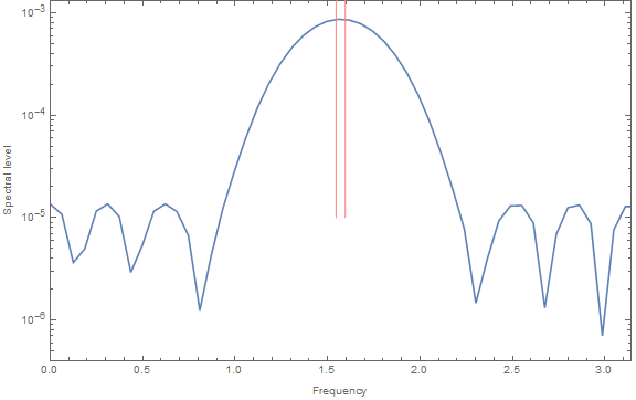
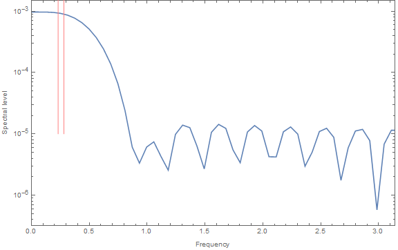
The first image shows a good bandpass filter. In the second image the center frequency is so small that the low frequency capability is lost. This is what happened to the poster.

I still think these filters should be used with caution because they are non-causal. They can result in output before there is input.

Answer 2

The difference between the low-high/high-low/bandpass filters is clearer plotting them all together:

lh = LowpassFilter[HighpassFilter[data, 0.01], 0.02]; 
hl = HighpassFilter[LowpassFilter[data, 0.02], 0.01]; 
b = BandpassFilter[data, {0.01, 0.02}];
ListPlot[{lh, hl, b}]

In fact, even the high-low and the low-high filtering are somewhat different (look around sample 300). One thing that is important in filtering is how large the filter is (how long the impulse response is). We can control this using the length parameter (the third argument) in the filters:

len = 50; 
lh = LowpassFilter[HighpassFilter[data, 0.01, len], 0.02, len]; 
hl = HighpassFilter[LowpassFilter[data, 0.02, len], 0.01, len]; 
b = BandpassFilter[data, {0.01, 0.02}, len];
ListPlot[{lh, hl, lh[[100]]/b[[100]] b}]

Now the low-high and high-lo are identical, and the bandpass is the same but for a scaling factor. The above code picks a single point (the 100th), and uses that to scale the bandpass.

Why does the length matter? The length is used to design the exact parameters of the filter -- longer filters allow closer approximations to the ideal filter shapes. When no length is specified, the algorithm picks a length based on some heuristics. The Details and Options section says that it "uses a filter kernel length and smoothing window suitable for the cutoff frequency and the input data." The heuristic is clearly picking different lengths in the low and high pass cases, and so presumably is also picking different values in the bandpass case as well.

Why the scale factor? When designing a filter, it is necessary to have some kind of gain specification -- this is an arbitrary constant that multiplies all parameters of the filter. For instance a common goal for a low pass filter is to set the gain at DC (zero frequency) to 1. A common goal for a high pass filter is to set the gain at infinity frequency to 1. But for a bandpass, you need to pick something else, because both of these are zero. I imagine they are setting some intermediate frequency gain equal to 1 (maybe at halfway between 0.1 and 0.2) but none of this is specified in the help file, so you would need to ask Wolfram.