5
$\begingroup$

To identify and classify the critical points of the function $f(x,y,z)=x^3+xz^2-3x^2+y^2+2z^2$, I used the Hessian matrix method.

Clear[f, x, y, z];
f = x^3 + x z^2 - 3 x^2 + y^2 + 2 z^2;
cpts = Solve[Grad[f, {x, y, z}] == 0, {x, y, z}, Reals]

This gave me the critical points $(0,0,0)$ and $(2,0,0)$. Then I calculate the Hessian.

H = D[f, {{x, y, z}, 2}];
MatrixForm[H]

Which gave me:

$$\begin{bmatrix} -6+6x & 0 & 2z\\ 0 & 2 & 0\\ 2z & 0 & 4+2z \end{bmatrix}$$

Then I calculated:

Det[H /. {x -> 2, y -> 0, z -> 0}]

Which was 96. Since this is positive, the Hessian method tells me that I must have a local minimum, maximum, or saddle point. Then I did this:

MatrixForm[H /. {x -> 2, y -> 0, z -> 0}]

Which gave me:

$$\begin{bmatrix} 6 & 0 & 0\\ 0 & 2 & 0\\ 0 & 0 & 8 \end{bmatrix}$$

Then the sequence of principal minors is:

$$ 6, \qquad \begin{vmatrix}6 & 0\\0 & 2\end{vmatrix}=12,\qquad\text{and}\qquad\begin{bmatrix}6 & 0 & 0\\0 & 2 & 0\\0 & 0 & 8\end{bmatrix}=96$$

Because they are all positive, we have a local minimum at (2,0,0). A similar test reveals a saddle point at (0,0,0).

My Question: I am now wondering how I might go about doing something in Mathematica to check that I do indeed have a local minimum, giving me some confidence in this method. Maybe something on the saddle point as well? I can't visualize due to the added dimension, but perhaps folks have some other ideas?

Notebook Share: This notebook will give you an idea of what I've written for my students thus far.

FindMinimum and FindMaximum Weird Result?

Trying belisarius and OleksandrR suggestion, I think I am looking at a very strange result:

In[12]:= FindMinimum[{f, (x - 2)^2 + y^2 + z^2 <= 1}, {x, 2}, {y, 
  0}, {z, 0}]

Out[12]= {-4., {x -> 2., y -> 0., z -> 0.}}

In[14]:= FindMaximum[{f, (x - 2)^2 + y^2 + z^2 <= 1}, {x, 2}, {y, 
  0}, {z, 0}]

Out[14]= {-4., {x -> 2., y -> 0., z -> 0.}}

Any thoughts or explanation on these results?

Michael E2 Comment Suggestion:

Since I am writing notebooks that have many pages, examples, and sometimes 2, 3, 4, or 5 Manipulate GUIs, I have to protect the content. So here is my adjustment to MichaelE2's wonderful example:

DynamicModule[{f, x, y, z, cpts},
 f = x^3 + x z^2 - 3 x^2 + y^2 + 2 z^2;
 cpts = {x, y, z} /. 
   Solve[Grad[f, {x, y, z}] == 0, {x, y, z}, Reals];
 Manipulate[
  With[{f0 = f /. Thread[{x, y, z} -> cp]}, 
   Show[ContourPlot3D[
     f == f0 + level, {x, cp[[1]] - 10^eps, cp[[1]] + 10^eps}, {y, 
      cp[[2]] - 10^eps, cp[[2]] + 10^eps}, {z, cp[[3]] - 10^eps, 
      cp[[3]] + 10^eps}, Mesh -> None, 
     PlotPoints -> ControlActive[9, 25],
     ContourStyle -> Opacity[0.7], 
     PlotLabel -> 
      Pane[Row[{"f \[Equal]", f0, 
         Sign[level] /. {-1 -> "-", 0 | 1 -> "+"}, Abs@level}, " "], 
       100]],
    Graphics3D[{
      Red, Sphere[cp, .04]
      }]
    ]],
  {{level, 0.}, -1., 1., Appearance -> "Labeled"},
  {{eps, 0., "zoom"}, -1, Log10[2.], Appearance -> "Labeled"},
  {cp, cpts}]]

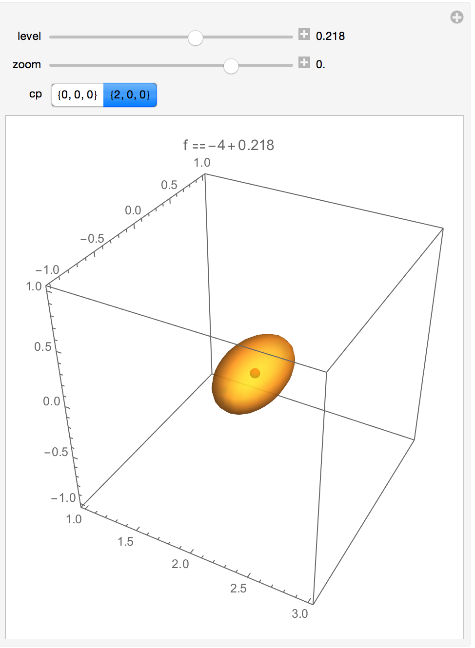
Adding ContourStyle->Opacity[0.7] and Graphics3D[{Red, Sphere[cp, .04]}] also shows the critical point.

enter image description here

$\endgroup$
7
  • $\begingroup$ NMinimize[f, {x, y, z}] finds your local minima $\endgroup$ Commented Aug 5, 2015 at 7:14
  • $\begingroup$ @belisarius FindMinimum is a better option for local minimization. Here you just happen to be lucky that NMinimize fails to find the global minimum. $\endgroup$ Commented Aug 5, 2015 at 10:19
  • $\begingroup$ @belisarius Check out the edit to my original post under FindMinimum and FindMaximum Weird Result? $\endgroup$
    – David
    Commented Aug 5, 2015 at 18:02
  • $\begingroup$ @David I wasn't the one who suggested FindMinimum :D $\endgroup$ Commented Aug 5, 2015 at 18:09
  • $\begingroup$ @David Re "Weird Result" -- The gradient is zero at the starting point, isn't it? It won't take a step. Try bumping the starting value by a small amount. $\endgroup$
    – Michael E2
    Commented Aug 6, 2015 at 3:08

3 Answers 3

2
$\begingroup$

If you want to teach the students to interpret level sets, then it is possible visualize the behavior of a function by manipulating the level. There are various ways to set it up, to cue the students' recognition of the type of extremum, etc. Here's one, whipped up rather quickly.

Clear[f, x, y, z];
f = x^3 + x z^2 - 3 x^2 + y^2 + 2 z^2
cpts = {x, y, z} /. Solve[Grad[f, {x, y, z}] == 0, {x, y, z}, Reals];
Manipulate[
 With[{f0 = f /. Thread[{x, y, z} -> cp]},
  ContourPlot3D[f == f0 + level,
   {x, cp[[1]] - 10^eps, cp[[1]] + 10^eps},
   {y, cp[[2]] - 10^eps, cp[[2]] + 10^eps},
   {z, cp[[3]] - 10^eps, cp[[3]] + 10^eps},
   Mesh -> None, PlotPoints -> ControlActive[9, 25],
   PlotLabel -> 
    Pane[Row[{"f \[Equal]", f0, Sign[level] /. {-1 -> "-", 0 | 1 -> "+"}, 
      Abs@level}, " "], 100]
   ]],
 {{level, 0.}, -1., 1.},
 {{eps, 0., "zoom"}, -1, Log10[2.]},
 {cp, cpts}]

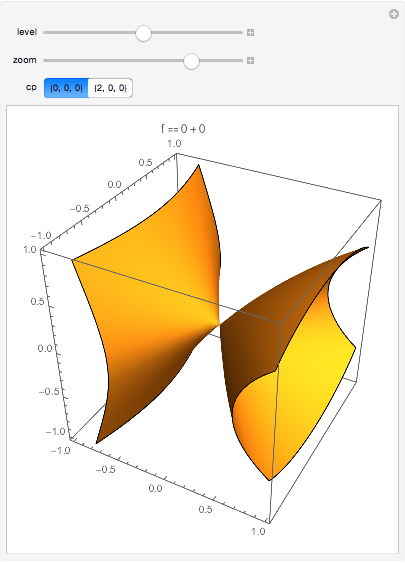
Example: This a typical picture of a saddle point. Move the level slider both left and right to see that f has values both less and greater than 0.

Mathematica graphics

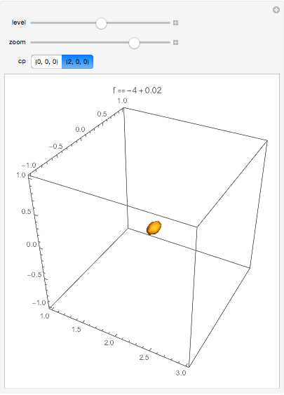
Example: f has a value greater than -4, so -4 is not a local maximum. Move the level to set it to a negative value to see that value below -4 is not possible (well, within the certainty of such numerical evidence).

Mathematica graphics

$\endgroup$
6
  • $\begingroup$ As usual, extremely helpful. Couple questions: 1) Is Contours->{{0}} needed? 2) In the Row command, what is the purpose of the " " at the end? 3) Why is the Pane command needed? 4) ControlActive[9,25} does what? Plot 9 points when dragging a slider, than 25 when you let go? $\endgroup$
    – David
    Commented Aug 6, 2015 at 3:55
  • $\begingroup$ As usual, if later in my notebook, I type Clear[f] or x=12, this Manipulate is ruined, so I've done the typical thing we've talked about in the past to make an adjustment. See my original post. What do you think? $\endgroup$
    – David
    Commented Aug 6, 2015 at 4:18
  • $\begingroup$ @David 1) You're right. I was playing with two different forms and forgot to remove it. 2) Look up Row; the 2nd arg is riffled between the row elements. 3) Pane keeps the label the same size so the it doesn't jump around when the number of digits change. 4) Look up ControlActive; it's for speed when the control is moved, and odd so that a sample point lies inside the ellipsoid-like figure at an extrema and the level is small and of the right sign (positive for {2,0,0} in the example). $\endgroup$
    – Michael E2
    Commented Aug 6, 2015 at 11:35
  • $\begingroup$ @David Looks good; global variables such as f etc. always present such pitfalls; localizing them is right approach and especially important when handing demonstrations off to independent humans to use (such as students). You might also be interested in this issue, mathematica.stackexchange.com/questions/90013/…, which came up while I played with your problem. $\endgroup$
    – Michael E2
    Commented Aug 6, 2015 at 11:40
  • $\begingroup$ If you don't have the time, please ignore this request. If you do, do you think you could add an update to this block of code based on your current work on http://mathematica.stackexchange.com/questions/84445/does-dynamicmodule-cure-problem-with-manipulate/90075#90075 ? It would be another great example to look at. $\endgroup$
    – David
    Commented Aug 7, 2015 at 19:51
6
$\begingroup$

another test:

f = x^3 + x*z^2 - 3*x^2 + y^2 + 2*z^2; 
cpts = Solve[Grad[f, {x, y, z}] == 0, {x, y, z}, Reals]

{{x -> 0, y -> 0, z -> 0}, {x -> 2, y -> 0, z -> 0}}

hesse = D[f, {{x, y, z}, 2}] /. cpts

{{{-6, 0, 0}, {0, 2, 0}, {0, 0, 4}}, {{6, 0, 0}, {0, 2, 0}, {0, 0, 8}}}

{ev1[l1,l2,l3], ev2[l1,l2,l3]} = Eigenvalues /@ hesse

{{-6, 4, 2}, {8, 6, 2}}

all eigenvalues positive -> local minimum

all eigenvalues negative -> local maximum

eigenvalues l1,l2,l3 with l1*l2*l3 < 0 -> saddlepoint

Completion

a further test

hesse matrix positive definit -> local minimum

hesse matrix negative definit -> local maximum

with Davids function:

f = x^3 + x*z^2 - 3*x^2 + y^2 + 2*z^2; 
cpts = Solve[Grad[f, {x, y, z}] == 0, {x, y, z}, Reals]
hesse = D[f, {{x, y, z}, 2}] /. cpts; 

{{x -> 0, y -> 0, z -> 0}, {x -> 2, y -> 0, z -> 0}}

PositiveDefiniteMatrixQ /@ hesse
NegativeDefiniteMatrixQ /@ hesse

{False, True}

{False, False}

-> first point = saddel, second point = local minimum

another function:

g = x^4 - y^4; 
pts = Solve[Grad[g, {x, y}] == 0, {x, y}]
h = D[g, {{x, y}, 2}] /. pts

{{x -> 0, y -> 0}}

{{{0, 0}, {0, 0}}}

PositiveDefiniteMatrixQ /@ h
NegativeDefiniteMatrixQ /@ h

{False}

{False}

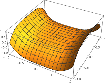
a saddle point

Plot3D[g, {x, -1, 1}, {y, -1, 1}]

plot3D

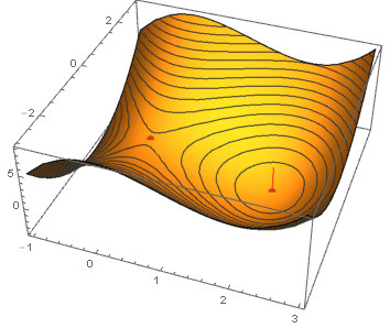
As an example, you can show your result:

f[x_, y_, z_] = x^3 + x*z^2 - 3*x^2 + y^2 + 2*z^2; 

Show[Plot3D[f[x, y, 0], {x, -1, 3}, {y, -3, 3}, 
     MeshFunctions -> {#3 & }], DiscretePlot3D[f[x, y, 0], 
     {x, {0, 2}}, {y, {0, 0}}, PlotStyle -> 
       Directive[Red, PointSize[Large]]]]

plot3d2

$\endgroup$
5
  • 1
    $\begingroup$ Yes, I did a little reading on positive and negative definite matrices, but these two tests and my test are the type of things that need rigorous abstract proofs in advanced classes. My question really wants to focus on whether there is any visual or numerical experimentation that can be done to verify that the answers given by my Hessian test are correct. $\endgroup$
    – David
    Commented Aug 5, 2015 at 16:48
  • $\begingroup$ "any visual … experimentation that can be done to verify that the answers given by my Hessian test are correct" - the quick visual test is to plot the quadratic form generated by truncating the Taylor expansion up to the Hessian term. A hyperbolic paraboloid means the point of the original function was a saddle; an elliptic paraboloid opening in the appropriate direction is what you'll get for an optimum. $\endgroup$ Commented Aug 5, 2015 at 17:08
  • $\begingroup$ @J.M. This could be something special I should learn. Perhaps you could do a detailed answer showing these results? Also, maybe you could point me toward some reading on this idea? $\endgroup$
    – David
    Commented Aug 5, 2015 at 18:04
  • $\begingroup$ I don't think I need to, @David. Look at Willinski's last figure, where he embedded contours in the surface to assist with the visualization. Note the hyperbola-like curves around the saddle and the ellipse-like curves around the optimum. There's your visual cue. :) $\endgroup$ Commented Aug 5, 2015 at 18:51
  • $\begingroup$ @Willinski. Thanks for that last image. I believe it very helpful. My assumption is that you assumed that the z-value of the critical point was zero, then searched for the x and y values. $\endgroup$
    – David
    Commented Aug 6, 2015 at 3:20
2
$\begingroup$

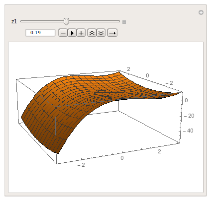
You can visualise a function of 3 paramters by putting one of them as argument of Manipulate:

Manipulate[Plot3D[f /. z -> z1, {x, -3, 3}, {y, -3, 3}], {z1, -3, 3}]

enter image description here

$\endgroup$
1
  • 1
    $\begingroup$ And how can I use this to demonstrate a local minimum at (2,0,0) and a saddle point at (0,0,0)? $\endgroup$
    – David
    Commented Aug 5, 2015 at 16:42

Your Answer

By clicking “Post Your Answer”, you agree to our terms of service and acknowledge you have read our privacy policy.

Not the answer you're looking for? Browse other questions tagged or ask your own question.