How to program efficient undershoot/overshoot

Question

I would like to solve the following boundary value problem for $y(x)$ for a fixed value of $k$ between $0 < k <1$:

$$y'' + \frac{3}{x} y' - y + \frac{3}{2}y^2 - \frac{k}{2}y^3=0 \\ y'(0) = 0,\qquad y(\infty)\rightarrow0$$

To make this work, I truncate the domain of the problem to $x_0 < x < x_\text{Max}$ to avoid the singularity at $x=0$ and so that the second boundary condition is brought to a finite $y(x_\text{Max})=0$. I will be working with $x_0 = 0.01$ and $x_\text{Max} = 10.$

I want to write a fast Mathematica program to solve this by using undershoot/overshoot on the related initial-value problem $y(x_0) = y_0$ to achieve the second boundary condition $y(x_\text{Max}) = 0$.

So far, I wrote a nice little code that solves the initial-value problem for a given $k$ and $y_0$:

sol = With[{x0 = .01, xMax = 10},
        ParametricNDSolveValue[
          {y''[x] + 3/x y'[x] - y[x] + 3/2 y[x]^2 - k/2 y[x]^3 == 0 (*diff.eq.*),
           y[x0] == y0 + 1/8 x0^2 (y0 - 3/2 y0^2 + k/2 y0^3)        (*init.cond.1*),
           y'[x0] == 1/4 x0 (y0 - 3/2 y0^2 + k/2 y0^3)              (*init.cond.2*),
           WhenEvent[y[x] == 0, {Print["Overshot"], "StopIntegration"}],
           WhenEvent[y'[x] == 0, {Print["Undershot"], "StopIntegration"}]
          },
          y, {x, x0, xMax}, {k, y0}]]

The solutions are obtained by calling sol[k,y0][x] and can be plotted by giving numbers for k and y0.

---

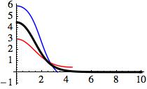
Example: Take $k=0.4$

Then, $y_0 = 6.0$ (blue) leads to an "overshoot", $y_0 = 3.0$ (red) leads to an "undershoot", and $y_0 = 4.51114$ (black) is the "sweetspot" which gives the solution to the boundary value problem.

Question: What is the best way (in terms of performance) to automate getting the solution to the boundary value problem in Mathematica?

I definitely know that the correct $y_0$ lies somewhere between $\frac{3-\sqrt{9-8k}}{2k} < y_0 < \frac{3+\sqrt{9-8k}}{2k}$.

---

Appendix: the following code generates the graphic above.

plot1 = Plot[sol[0.4, 6][x], {x, .01, sol[0.4, 6]["Domain"][[1, 2]]}, PlotStyle -> Blue];
plot2 = Plot[sol[0.4, 3][x], {x, .01, sol[0.4, 3]["Domain"][[1, 2]]}, PlotStyle -> Red];
plot3 = Plot[sol[0.4, 4.51114][x], {x, .01, sol[0.4, 4.51114]["Domain"][[1, 2]]}, PlotStyle -> {Black, Thick}];
Show[plot1, plot2, plot3, PlotRange -> {{0, 10}, {-1, 6}}]

Answer 1

A mundane but effective approach is to use the Shooting Method built into NDSolve.

x0 = .01; xMax = 11.5; k = .4;
c = N[D[(BesselK[1, x]/x), x]/(BesselK[1, x]/x) /. x -> xMax];
sol = NDSolveValue[{y''[x] + 3/x y'[x] - y[x] + 3/2 y[x]^2 - 
     k/2 y[x]^3 == 0, y'[xMax] == c y[xMax], y'[x0] == 0}, y, {x, x0, xMax}, 
  Method -> {"Shooting", "StartingInitialConditions" -> {y[x0] == 4.5, y'[x0] == 0}}]

Note that the boundary condition y'[xMax] == c y[xMax] is employed to match the exponentially decreasing asymptotic solution to the ODE, BesselK[1, x]/x. Also, xMax is increased to 11.5.

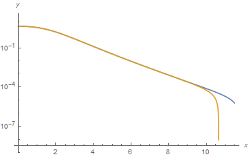
The k = .4 solution, compared to that given in the question is,

LogPlot[{sol[x], solt[x]}, {x, x0, xMax}, AxesLabel -> {x, y}]

Two features are evident. First, the solution already is exponentially decreasing at x = 3. Second, both approaches become unstable, the method in the Question at about x = 9.5 and that given here at about x = 11. This presumably occurs due to unavoidable round-off errors that couple into the second, exponentially growing, asymptotic solution to the ODE.

The value of y near the origin agrees quite closely with that in the Question.

sol[x0]
(* 4.51095 *)

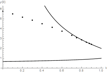
The next plot depicts y[x0] (points) as a function of k, along with the bounds on y[x0] (solid curves) given in the Question. (These bounds correspond to the values of y[x0] which satisfy the ODE for all x, apart from the boundary condition at infinity.)

data = {{0., 5.78018}, {0.1, 5.49104}, {0.2, 5.18459}, {0.3, 4.85871}, {0.4, 4.51095}, 
        {0.5, 4.13862}, {0.6, 3.73916}, {0.7, 3.31151}, {0.75, 3.08818}, 
        {0.8, 2.86076}, {0.85, 2.63322}, {0.88, 2.49923}, {0.9, 2.41187}};
Show[ListPlot[data, AxesLabel -> {"k", y[0]}, PlotStyle -> Black], 
  Plot[{(3 - Sqrt[9 - 8 k])/(2 k), (3 + Sqrt[9 - 8 k])/(2 k)}, {k, 0, 1},
  PlotStyle -> Black], PlotRange -> {{0, 1}, {0, 6}}]

Solutions for k < .8 are obtained with moderate ease by first running the code above with xMax = 5, which is fairly forgiving of inaccurate initial guesses for y[x0], and then using the resulting actual y[x0] with xMax = 10 to obtain y[x0] accurate to five significant figures or better. The process becomes rather more delicate at larger k, because y[0] lies very close to its upper bound. I typically would need to guess about five times (moving the point at which NDSolve declared the equations stiff toward xMax) and also increase xMax somewhat to obtain a solution that was both stable and accurate. Any particular calculation takes less than a second of computer time.

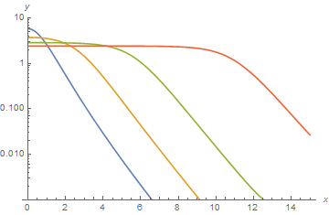
A comparison among y for k of 0(blue), .6(brown), .8(green), and .9 (red) follows. That the k = 0.9 solution is essentially constant out to about x = 10 explains why the calculation at larger k is so delicate and also why xMax = 15 is necessary for accuracy.

Note that I have not experimented with NDSolve Methods for handling stiffness, which may improve the robustness of this solution. Nonetheless, I was able to obtain the curves above without excessive difficulty.