Nonlinear differential equation: numerical solution

Question

I have to find and plot a numerical solution for this second order differential equation:

u''[x] + (u'[x]/x) - (u[x]/(x^2)) + u[x] - u[x]^3 = 0

where $0\leq x < \infty$ and $u(x=0)=0$, $\lim\limits_{x\to\infty}u(x)=1$. How can I do it? Thank you very much.

Answer 1

Introduction

I think there are several questions on this site about ODEs of the form $$(x-a)^2 u''(x) = F(x,u,u')$$ with an initial condition at $x=a$.

There is no general guarantee that solutions exist over an interval $(a,b]$, but sometimes it is possible as in this case.

Outline

We transform the equation $u''(x) = F(x,u,u')$ over the infinite interval $[0, \infty)$ into an equation $v''(t)= G(t,v,p=v')$ over to the finite interval $[0,1]$. Thus we will transform the OP's problem into a BVP with boundary conditions $v(0)=0$, $v(1)=1$.

Looking at the power series expansion, we discover that $v(0)=0$ is a necessary condition and that $v'(0)=p_0$ is a free variable. This is encouraging in that there is a degree of freedom in trying to get the boundary condition $v(1)=1$ satisfied. It turns out that at $t=1$ ($x=\infty$), there are three critical points $(v, p) = (-1,0),\ (0,0),\ (1,0)$. The one at $(1,0)$ is unstable, but at least it might be possible to meet the boundary conditions.

We present two methods of solution, one a sort of finite element method and the other a shooting method. Each uses the conditions imposed by the boundary conditions.

Transformation to a finite interval

The interval of integration $[0,\infty)$ may be transformed to $[0,1)$ by the substitution $x = t/(1-t)$.

uxeq = u''[x] + (u'[x]/x) - (u[x]/(x^2)) + u[x] - u[x]^3;

xsub = First@ Solve[{v[t] == u[x[t]], p == D[u[x[t]], t],
  q == D[u[x[t]], t, t]}, {u[x[t]], u'[x[t]], u''[x[t]]}] /. {p -> v'[t], q -> v''[t]};

xf = #/(1 - #) &;
tf = #/(1 + #) &;
With[{v2 = First@ Solve[uxeq /. x -> x[t] /. xsub /. x -> xf // Factor // # == 0 &, v''[t]]},
  vtRHS = v''[t] /. v2];
vteq = v''[t] == vtRHS

$$v''(t)={1 \over (t-1)^4 t^2}\,\left({ (1-2 t)\, v(t)+t^2\, v(t)^3 - t \, (2 t-1) (t-1)^3\, v'(t)}\right)$$

Analysis of the ODE

The power series expansion about $t=0$ of the ODE

Series[v''[t] - vtRHS, {t, 0, 1}]

$$-\frac{v(0)}{t^2}-\frac{2 v(0)}{t}+\left(\frac{3 v''(0)}{2}-3 v'(0)-v(0)^3-2 v(0)\right)+t \left(\frac{4}{3} v^{(3)}(0)-2 v''(0)-3 v(0)^2 v'(0)-3 v'(0)-4 v(0)^3\right)+O\left(t^2\right)$$

shows that the singularity vanishes when $v(0)=0$.

Series solution code

The following returns a list of replacement rules for the derivatives of a solution to the ode satisfying the initial condition ic. The argument iter should be of the form {t, t0, n}, similar to the command Series, This is used in the OP's problem to discover any conditions imposed on higher derivatives by the boundary conditions.

seriesDSolve[ode_, iter_, ic_: {}] := Fold[
  Flatten[{#1, Solve[#2 == 0 /. #1]}] &,
  ic,
  Series[ode /. Equal -> Subtract, iter][[3]]
  ]

Series expansion of the ODE

There are singularities at the end points of the interval $[0,1]$, a pole of order 2 at $0$ and a pole of order 4 at $1$.

If we examine the solutions with initial condition $v(0)=0$, we see that, at least locally, the first derivative $v'(0)$ is a free variable.

seriesDSolve[v''[t] - vtRHS, {t, 0, 2}]

At the initial condition $v(1)=1$, all the derivatives $v^{(n)}(1)$ seem to be determined. In other words, there seem to be no degrees of freedom.

seriesDSolve[v''[t] - vtRHS, {t, 1, 0}, v[1] -> 1]

The one degree of freedom at the initial condition $v(0)=0$ would allow for the possibility of a shooting method approach with the parameter $v'(0)=p_0$ to finding a solution to the OP's boundary value problem.

Solutions

We'll show two numerical solutions to the transformed differential equation in $v$ over $0 \le t \le 1$, a sort of nonlinear finite element method and a shooting method. In each case, we'll use the power series expansion to help satisfy the boundary condition at t == 0. In the finite element approach we will mesh the interval $[0,1]$ and use the nonlinear solver FindRoot to approximate the differential equation at the mesh points. In the shooting method, we will use the power series to determine the initial step at the boundary condition $v(0)=0$. The boundary condition $v(1)=1$ is an unstable equilibrium and there will be a limit to how close a solution may approach $t=1$. We will return a solution that maximizes how far the integration was carried out, taking advantage of the characteristics of the instability of around $v(1)=1$ to determine stopping criteria for the integration.

There are advantages and disadvantages to each method. The finite element method gives a solution to the original differential equation that may be computed for any $x$ in the interval $0<x<+\infty$, whereas the shooting method can compute a solution only up to $x$ equal to $14$ to $40$ depending on the working precision (from machine precision to 100 digits resp.) On the other hand the automatic controls in NDSolve make the shooting method solution track the differential equation more closely than the finite element method. That leads to the problem of an optimal mesh, which we will not investigate here.

In both methods we make use of a function rhsFN, which is equal to the right-hand side vtRHS of the ODE for $0<t<1$. At the end points $t=0$ and $t=1$, we impose the boundary conditions in the definition of rhsFN from the series expansion of v''[t] - vtRHS; the value v'[0] -> p0is a free parameter and an argument to rhsFN.

Clear[rhs];
Block[{p0, t},
 rhsFN[p0_][t_] = Piecewise[{{vtRHS, t != 0 && t != 1}, {2 p0, t == 0}}, 0];
 ]

Nonlinear "finite element" method

The basic procedure is as follows:

• Mesh the interval.
• Set up the differential equation as a system of first-order equations of the form $(y, p,\dots)'=f(t,y,p,\dots)$, where $p = y'$ etc.
• Create an array of variables, one for each dependent variable in the differential equation per mesh point.
• Load the boundary conditions into the array; also load any other conditions entailed on the variables by the power series expansions at the boundary points.
• Set up the system of equations, given by the differential equation at each point of the mesh; the derivatives $(y, p,\dots)'$ of the left-hand side are approximated by finite differences.
• Solve the system.

The OP's BVP

The OP's ODE is equivalent to the system

{v'[t] == p[t], p'[t] == vtRHS /. v'[t] -> p[t]}
(*
  {v't] == p[t],
   p'[t] == (1/((-1 + t)^4 t^2)) *
     (-t p[t] + 5 t^2 p[t] - 9 t^3 p[t] + 7 t^4 p[t] - 2 t^5 p[t] +
      v[t] - 2 t v[t] + t^2 v[t]^3)}
*)

My trials showed that using a uniform mesh of the interval 0 <= t <= 1 seems to undersample near the singularities at the end points (and oversample in the middle). So I add some additional points near the end points. The values of the variables $v=v(t)$ and $p=v'(t)$ are stored in the arrays vvals and pvals respectively. Except for the values entailed by the boundary conditions, these are free variables v[i] and p[i] respectively. These values and variables can then be loaded into the right-hand side of the system above. The left-hand side is computed from the values using NDSolve`FiniteDifferenceDerivative. The singular end points have to be handled separately (hence the 2 ;; -2 in the code).

(* set up *)
tgrid = Sort@
   Join[Range[0., 1., 1./256], 1./512 + Range[0., 0.9, 1./256],
    Range[7]/8./512., 1. - Range[7]/8./256., 1. - Range[7]/8.^2/256.];
vvals = Table[If[i == 1, 0., If[i == Length@tgrid, 1., v[i]]], {i, Length@tgrid}];
pvals = Table[If[i == Length@tgrid, 0., p[i]], {i, Length@tgrid}];

Block[{t, v, p, p0},
 rhsFEM = Function[{t, v, p, p0},
   Evaluate@ {p, rhsFN[p0][t] /. {v[t] -> v, v'[t] -> p}}]
 ]

rhs = Transpose@ MapThread[
    rhsFEM[##, p[1]] &,
    {tgrid[[2 ;; -2]], vvals[[2 ;; -2]], pvals[[2 ;; -2]]}
    ];
lhs = {NDSolve`FiniteDifferenceDerivative[1, tgrid, vvals][[2 ;; -2]],
   (lhs1 = First[#]; Rest[#]) &@
    NDSolve`FiniteDifferenceDerivative[1, tgrid, pvals][[1 ;; -2]]};

The NDSolve` context contains a function ScaledVectorNorm for measuring the scaled error with respect to a solution vector for a given precision and accuracy.

svn = NDSolve`ScaledVectorNorm[2, {1.`*^-6, 1.`*^-6}];

A value of ScaledVectorNorm less than 1 indicates that the precision/accuracy goal has been met. Since we do not have an exact solution, we'll test the difference between the left and right-hand sides with respect to the right-hand side.

Machine-precision solution via FindRoot. I just use a line between the boundary points as a starting solution; that is, it gives the initial guesses for the values for the variables v[i] and p[i].

(* Machine-precision solution *)
vsol = v -> Interpolation[{{0., 0.}, {1., 1.}}, InterpolationOrder -> 1];
With[{
  v0 = Clip[v[tgrid] /. vsol, {0., 1.}],
  p0 = v'[tgrid] /. vsol},
 {sol = FindRoot[
       Flatten@ {lhs1 - 2 p[1], lhs - rhs},
       Join[Table[{v[i], v0[[i]]}, {i, 2, Length@tgrid - 1}],
        Table[{p[i], p0[[i]]}, {i, 1, Length@tgrid - 1}]]
       ]; // AbsoluteTiming // First,
  svn[Flatten[lhs - rhs] /. sol, Flatten[rhs] /. sol]}
 ]
vsol = v -> Interpolation@Transpose[{List /@ tgrid, vvals, pvals} /. sol];

FindRoot::lstol: The line search decreased the step size to within tolerance specified by AccuracyGoal and PrecisionGoal but was unable to find a sufficient decrease in the merit function. You may need more than MachinePrecision digits of working precision to meet these tolerances. >>

(*  {0.223435, 25219.2}  *)

Interestingly, the numerics trouble is in calculating the error, not in finding the roots. If we feed arbitrary-precision numbers to svn, we set that the error is quite good (much less than 1):

With[{nsol = sol /. x_Real :> SetPrecision[x, 15],
  r = rhs /. x_Real :> SetPrecision[x, 15],
  l = lhs /. x_Real :> SetPrecision[x, 15]},
 svn[Flatten[l - r] /. nsol, Flatten[r] /. nsol]
 ]
(*  0.0388375  *)

If we set up the solution with a WorkingPrecision of 16 or higher, we do not get the warning message from FindRoot, but the solution is not really any better. Refining the mesh tgrid would be a better approach to reducing error in the solution.

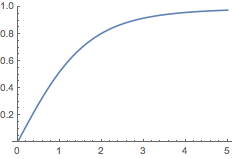
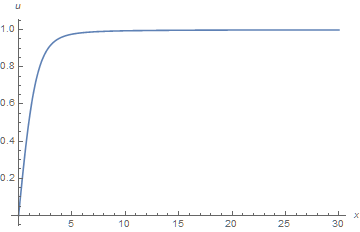
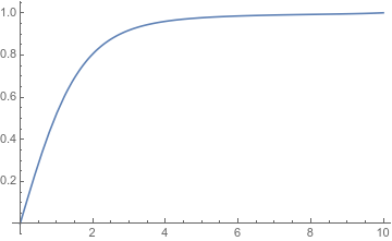
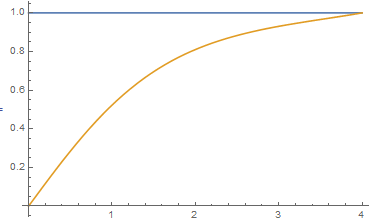
Plot[v[tf[x]] /. vsol, {x, 0, 5}]
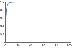
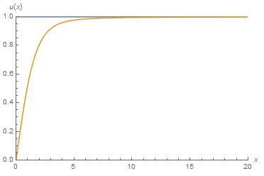
Plot[v[tf[x]] /. vsol, {x, 0, 100}]

Shooting method

The basic procedure is as follows.

• Identify necessary constraints and free variables in the power series expansion at the initial condition.
• If useful, identify necessary constraints in the variables at the other boundary condition. -- This is unnecessary in the current problem; the boundary is not reached in practice.
• Construct functions for the variables that meet the constraints at the boundary conditions.
• Construct a ParametricFunction whose parameters are the free variables at the initial condition and which stops integration when it begins to diverge from the target boundary value (see below for further discussion).
• Choose starting initial values for the variables and maximize the interval of integration.

The divergence criteria are dependent on properties that the OP's system has.

The OP's BVP

The boundary conditions are included in the construction of the function rhsFN, which represents the right-hand side of the ODE and which has been given above.

The idea is to use the parameter v'[0] == p0 to shoot as close to the boundary condition v[1] == 1 as possible. There are two ways to tell when a solution is beginning to diverge from the boundary condition. One is that v[t] > 1, after which the solution would go to infinity (provided t is larger than 1/2 in the OP's case, which is not checked, since such an integral curve is far from the desired curve and stopping when v[t] > 1 does not obstruct finding a solution). The other is that v'[t] < 0, provided v[t] < 1, after which the solution enters an oscillation around v[t] == 0.

We set up the shooting method with ParametricNDSolve and an objective function objmp that returns the time the NDSolve integration stopped. The objective function will be maximized.

psolmp = ParametricNDSolveValue[
  {v''[t] == rhsFN[p0][t], v[0] == 0, v'[0] == p0,
   WhenEvent[v'[t] < 0, "StopIntegration"],
   WhenEvent[v[t] > 1., "StopIntegration"]},
  v, {t, 0, 1}, {p0}]

Clear[objmp];
objmp[p0_?NumericQ] := psolmp[p0]["Domain"][[1, -1]]

We should give FindMaximum starting value. The value p0 == 1 is a reasonable first guess as it is the average slope between the boundary conditions.

({tmaxmp, parammp} = FindMaximum[objmp[p0], {p0, 1}]) // AbsoluteTiming
vsolmp = v -> psolmp[p0 /. parammp];
xf[tmaxmp]

FindMaximum::sdprec: Line search unable to find a sufficient increase in the function value with MachinePrecision digit precision. >>

(*
  {0.553742, {0.927063, {p0 -> 0.583184}}}  timing, tmax, sol
  12.7104                                   max x
*)

It's a good start, but given the singularities at the endpoints, one should expect that higher precision may be needed, especially near $t=1$. The previous solution gives an estimate for p0 (in parammp).

We can bump up WorkingPrecision to extend the interval for the solution.

psol = ParametricNDSolveValue[
  {v''[t] == rhsFN[p0][t], v[0] == 0, v'[0] == p0,
   WhenEvent[v'[t] < 0, "StopIntegration"],
   WhenEvent[v[t] > 1., "StopIntegration"]},
  v, {t, 0, 1}, {p0}, PrecisionGoal -> 12, AccuracyGoal -> 12,
  WorkingPrecision -> 100]

Clear[obj];
obj[p0_?NumericQ] := psol[p0]["Domain"][[1, -1]]

Using the value for p0 from the MachinePrecision computation, we can give two starting values to avoid computing derivatives. This gives a solution out to x == 40+ (t == 15.4).

({tmax, param} =
   FindMaximum[obj[p0], {p0, 0.582`100, 0.583`100},
    PrecisionGoal -> 12, AccuracyGoal -> 12,
    WorkingPrecision -> 100]) // AbsoluteTiming
vsol = v -> psol[p0 /. param];
xf[tmax]
(*
  {15.4183, {0.9760616528..., {p0 -> 0.5831894926...}}}
  40.7739
*)

Or we could give the value directly. The result is a little better (if we bracket the solution), but it takes a lot longer.

p0mp = p0 /. param
({tmax, param} =
   FindMaximum[obj[p0], {p0, p0mp, p0mp - 0.1, p0mp + 0.1},
    PrecisionGoal -> 12, AccuracyGoal -> 12,
    WorkingPrecision -> 100]) // AbsoluteTiming
vsol = v -> psol[p0 /. param];
xf[tmax]

FindMaximum::lstol: The line search decreased the step size to within the tolerance specified by AccuracyGoal and PrecisionGoal but was unable to find a sufficient increase in the function. You may need more than 100.` digits of working precision to meet these tolerances. >>

(*
  {355.47, {0.9781137344..., {p0 -> 0.5831894926...}}}
  44.6907
*)

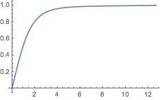
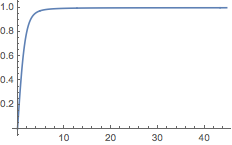
Each produces a reasonable plot:

Plot[v[tf[x]] /. vsolmp, {x, 0., xf[tmaxmp]}, PlotRange -> All]
Plot[v[tf[x]] /. vsol, {x, 0., xf[tmax]}, PlotRange -> All]

Answer 2

This question seeks the separatrix of a nonlinear ODE over the range {0, Infinity}. As noted by Michael E2, many such problems have been presented on this site. (Personally, I have answered 97492, 97238, 84131, and 77981.) They are difficult not only due to the infinite range but also because integrating along the separatrix is inherently numerically unstable: slight errors typically lead to exponential departures from the separatrix.

One approach to solving the ODE without a transformation of variables is to approximate the asymptotic solution by a series in x^-1

n = 20; app = Sum[a[i] x^-i, {i, 0, n}];
Unevaluated[1/x D[x D[u[x], x], x] - (u[x]/(x^2)) + u[x] - u[x]^3] /. u[x] -> app;
CoefficientList[Series[%, {x, Infinity, n}] // Normal, 1/x];
exp = app /. Solve[Thread[% == 0], Array[a[# - 1] &, n + 1]][[3]];

(The first few terms are 1 - 1/(2 x^2) - 1/(8 x^4).) The series is not alternating.

Then the ODE is solved numerically over the range {x0, inf}, here

x0 = 10^-10; inf = 30;
s = ParametricNDSolveValue[{1/x D[x D[u[x], x], x] - (u[x]/(x^2)) + u[x] - u[x]^3 == 0,
    u[x0] == 0, u'[x0] == b}, u, {x, x0, inf}, {b}, WorkingPrecision -> 30];

and the parameter b obtained by matching s[b][inf] to exp /. x -> inf. However, for too large a value for b, the integration of s[b] terminates early. The range over which the integration runs to inf can be determined quickly from

bl = 1; bu = 1.2;
Do[bt = (bl + bu)/2; If[Quiet@s[bt]["Domain"][[1, 2]] < inf, bu = bt, bl = bt], {i, 60}]
NumberForm[{bl, Quiet@s[bl]["Domain"][[1, 2]], bu, Quiet@s[bu]["Domain"][[1, 2]]}, 18]
(* {1.1663789917200773, 30.0000000000000000, 1.1663789917200775, 29.2709289364276124} *)

after which

b0 = b /. FindRoot[s[b][inf] == exp /. x -> inf, {b, 1.15, bl}, WorkingPrecision -> 30]
(* 1.16637899172007724729860894319 *)

Finally, the numerical solution is for x < inf is

Plot[{s[b0][x]}, {x, x0, inf}, AxesLabel -> {x, u}, PlotRange -> All]

and the series solution used for larger values of x. Some feel for the error involved in this approach can be obtained from

err = -exp[[2]]; LogPlot[{exp - s[b0][x], exp - s[b0ld][x], err}, {x, 10, inf}, 
    AxesLabel -> {x, Δu}, PlotRange -> {10^-16, 10^-8}]

The blue curve is the difference between the numerical and series solutions for x < inf. (Noise near r = inf shows the accuracy limitations of WorkingPrecision -> 30.) The orange curve is the same quantity computed for inf = 20.

b0ld = 1.16637899172007724729865778156

In all, the errors are acceptably small. (The green curve is an error estimate, equal to the negative of the x^-20 term in the series.) Finally, for completeness, the distance at which the s[b] integration halts is given by

Plot[Quiet@s[b]["Domain"][[1, 2]], {b, 1.16, 1.17}, AxesLabel -> {b, x}, 
    Epilog -> {PointSize[Large], Red, Point[{b0, inf}]}, PlotRange -> All]

Superimposed as a red point is b0. The FindRoot computation above takes place on the flat region of the curve. Apart from determining the last plot, the total time for this computation is about one minute on my PC.

Edit: Literature Search

The ODE is Bessel's nonlinear differential equation of order one. Many articles have been published on it and its generalizations, although I have not yet found any discussing numerical methods in detail. Search, for instance, Google for "nonlinear Bessel equation".

Answer 3

In version 12 you can use:

inf = 10;
sol = NDSolveValue[{u''[x] + (u'[x]/x) - (u[x]/(x^2)) + u[x] - 
     u[x]^3 == 0, DirichletCondition[u[x] == 0, x == 0], 
   DirichletCondition[u[x] == 1, x == inf]}, u, {x, 0, inf}, 
  Method -> {"FiniteElement", 
    "MeshOptions" -> {"MaxCellMeasure" -> 0.01}}, 
  InitialSeeding -> {u[x] == 1}]

For this type of (Ginzburg-Landau) equation it's needed to give an initial seeding away from 0 (which is the default). The solution gives messages that the solution may be unstable:

NDSolve`FEM`InitializePDECoefficients::femcsdp: The product of 2 times the Damkoehler number (2.0000999999996028`) and the Peclet number (0.9999999999998012`) is 4.00019999999841` and is larger than the mesh order (2), and the computed result may not be stable. Adding artificial diffusion may help.

NDSolve`FEM`InitializePDECoefficients::femcsdp: The product of 2 times the Damkoehler number (2.0000999999996028`) and the Peclet number (0.9999999999998012`) is 4.00019999999841` and is larger than the mesh order (2), and the computed result may not be stable. Adding artificial diffusion may help.

However, the solution looks fine:

Plot[sol[x], {x, 0, inf}, PlotRange -> All]

Answer 4

By advice @Alexei Boulbitch,but works only for interval 0 < x < 4.

 sol = With[{ϵ = 1/1000000}, 
 First@NDSolve[{u''[x] + u'[x]/x - u[x]/x^2 + u[x] - u[x]^3 == 0, 
 u[ϵ] == 0, u[4] == 1}, u[x], {x, ϵ, 4}, 
 Method -> {"ExplicitRungeKutta", "DifferenceOrder" -> 5}, 
 InterpolationOrder -> All]];

 Plot[{1, Evaluate[u[x] /. sol]}, {x, 0, 4}]

EDITED !!!

Or we can use a inital condition u'[20]=1.166380071748 calculated with "brute force".

 sol = With[{ϵ = 1/1000000000000, ϵ2 = 20}, 
 NDSolve[{u''[x] + u'[x]/x - u[x]/x^2 + u[x] - u[x]^3 == 0, 
 u[ϵ] == 0, 
 u'[ϵ] == Rationalize[1.166380071748, 0]}, 
 u, {x, ϵ, ϵ2}, WorkingPrecision -> 16]];
 Plot[{1, u[x] /. sol}, {x, 1/1000000000000, 20}, 
 PlotRange -> {{0, 20}, {0, 1}}, AxesLabel -> {x, u[x]}]