How to combine 2d and 3d plots with this code [duplicate]

Question

I found a picture for example in google and I want to do with my code like that:

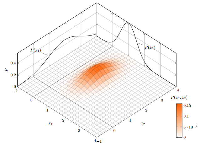
And here is my code:

\[CapitalOmega] = Rectangle[{0, 0}, {1, 1}];
op = Laplacian[u[x, y], {x, y}] + 2;
Subscript[\[CapitalGamma], 
D] = {DirichletCondition[u[x, y] == 0, True]};
\[CapitalPhi] = 
NDSolveValue[{op == 0, Subscript[\[CapitalGamma], D]}, 
u, {x, y} \[Element] \[CapitalOmega]];
Plot3D[\[CapitalPhi][x, y], {x, y} \[Element] \[CapitalOmega], 
PlotStyle -> None]

Answer 1

Use ParametricPlot3D to create the integrated curves as parametric curves along the lines {x,1} and {y,0}. Then use Show to combine the objects together.

\[CapitalOmega] = Rectangle[{0, 0}, {1, 1}];
op = Laplacian[u[x, y], {x, y}] + 2;
Subscript[\[CapitalGamma], D] = {DirichletCondition[u[x, y] == 0, True]};
\[CapitalPhi] = NDSolveValue[{op == 0, Subscript[\[CapitalGamma], D]}, u, {x, y} \[Element] \[CapitalOmega]];
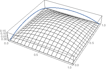
graph1 = Plot3D[\[CapitalPhi][x, y], {x, y} \[Element] \[CapitalOmega], PlotStyle -> None]
xint[y_] := Integrate[\[CapitalPhi][x, y], {x, 0, 1}]
yint[x_] := Integrate[\[CapitalPhi][x, y], {y, 0, 1}]
Show[ParametricPlot3D[{0, y, xint[y]}, {y, 0, 1}], 
ParametricPlot3D[{x, 1, yint[x]}, {x, 0, 1}], graph1, 
PlotRange -> {{0, 1}, {0, 1}, All}]

Result: