Well, numerical approach is at least straight forward, though maybe a bit tedious to make perfectly automated. Here is a crude start. I will deal only with real part of your function. Find the table of points and flip point pairs:
invf = Re@Table[{f[r], r}, {r, 0.001, 5, .01}];
gr = Show[ListLinePlot[invf, PlotStyle -> Red],
 Plot[{r, Re@f[r]}, {r, 0, 5}], AspectRatio -> 1,
 PlotRange -> {{0, 5}, {0, 5}}, Frame -> True, Axes -> False]
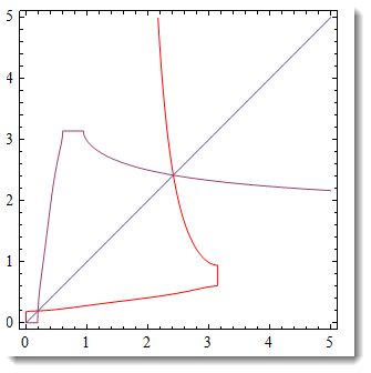
What follow is a bit manual. You see in this case you have 2 branches. Split your function for each of them. Of course this is just a start, you can explore further.
invff1[r_] := (Sort[Transpose[{Abs[#[[All, 1]] - r], #[[All, 2]]}]] &@
     Select[invf, #[[2]] < .8 &])[[1, 2]];
invff2[r_] := (Sort[Transpose[{Abs[#[[All, 1]] - r], #[[All, 2]]}]] &@
     Select[invf, #[[2]] > .8 &])[[1, 2]];
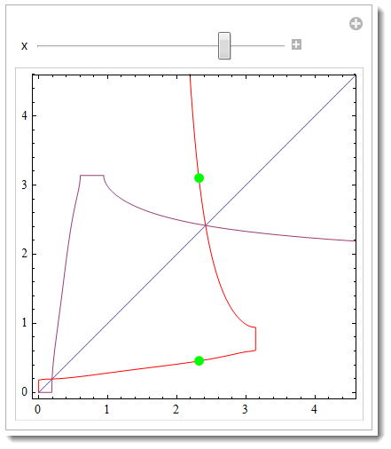
You have to be careful with ranges. Limit the ranges to what your data are well defined for and you basically got yourself an inverse function:
Manipulate[
 Show[gr,
  Graphics[{Green, PointSize[.03], Point[{x, invff1[x]}],
    Point[{x, invff2[x]}]}], PlotRange -> {{0, 4.5}, {0, 4.5}}]
 , {x, 0, 3}, FrameMargins -> 0]
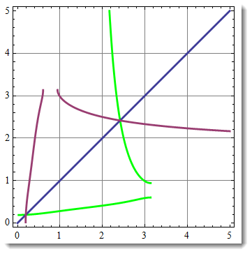
Following @J.M. comment adding ParametricPlot[] way of looking at inverse:
Show[ParametricPlot[{f[r], r}, {r, 0.1, 5}, PlotStyle -> Green],
 Plot[{r, f[r]}, {r, 0, 5}], AspectRatio -> 1,
 PlotRange -> {{0, 5}, {0, 5}}, Frame -> True, Axes -> False,
 GridLines -> Automatic, BaseStyle -> Thick]


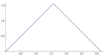
Solve[Cos[s] == (* stuff inside the ArcCos[] *), r], but that yields a bunch ofRoot[]objects, and you need to pick which solution is appropriate... $\endgroup$g = Solve[ Cos[s] == (-1 + 4.20278 r (0.008712/r^2 + 0.475876/r - 1/(1 + r)))/ Sqrt[1 - 10.598 r^2 (0.008712/r^2 + 0.475876/r - 1/(1 + r))], r]; Show[Plot[r /. g[[3]], {s, 0, \[Pi]/2}, PlotRange -> {{0, \[Pi]}, {0.15, 0.65}}], Plot[r /. g[[4]], {s, \[Pi]/2, \[Pi]}]]$\endgroup$