Seeking simple function in interval

Question

I am a bit rusty, and struggling to solve this problem. Looking for a simple, well behaved parametric function f[t], from [0,1] to [0,1] such that:

f[0] = f0;

f[1] = f1;

f'[1] = ff1; where -1<= ff1 <0

(NOTE: the latter condition make the problem hard if f1 is very close to 1 and ff1 is quite strongly negative).

and ideally, I would also like: f'[0] = 0 (or ff0) and f unimodal in [0,1].

The latter condition probably rules out rational functions, which would be a pity as the parameters might have to be computed often given the f0,f1, etc, and Solve does not seem to like trascendantal functions because of the condition on f'.

I would like it to have an additional free parameter, some sort of "scale", that allows to control how quickly f[t] changes from the region close to 0 to the region close to 1. I understand from Artes comments that complex conditions can be added to Solve using Exists, BUT I still cannot find a solution.

Any suggestions appreciated. Thanks!

EDIT: removed the example as it generated confusion, and tried to clarify the conditions. Added a note.

Answer 1

EDIT 05.04.14 / 04.12.14

Let us consider a function of the form

f[x_] = v[x]^2/(1+v[x]^2)

with

v[x_] = a + b x + c x^2 + d x^3

Then

(i) f is in [0,1)
(ii) because

f'[x] = (2 v[x] v'[x])/(1 + v[x]^2)^2

there are at most two extreme values of f[x], at the zeroes of v'[x] which are at

x+- = (-c +- Sqrt[c^2 - 3 b d])/(3 d)

Their position can be controlled by the parameter d.

The function v[x] is given explicitly through the boundary values (f0, f1, f11) by

v[x_] = Sqrt[f0]/Sqrt[
 1 - f0] + (d - (2 Sqrt[f0])/Sqrt[1 - f0] + (2 Sqrt[f1])/Sqrt[
    1 - f1] - (Sqrt[f1] f11)/(2 Sqrt[1 - f1] (f1 - f1^2))) x + (-2 d +
     Sqrt[f0]/Sqrt[1 - f0] - Sqrt[f1]/Sqrt[1 - f1] + (Sqrt[f1] f11)/(
    2 Sqrt[1 - f1] (f1 - f1^2))) x^2 + d x^3

and f[x] correspondingly.

Derivation of v[x]:

The boundary values of v[x] in terms of those of f[x] are given by

Solve[{f[0] == f0, f[1] == f1, f'[1] == f11}, {v[0], v[1], v'[1]}]

(* {{v[0] -> -(Sqrt[f0]/Sqrt[1 - f0]), v[1] -> -(Sqrt[f1]/Sqrt[1 - f1]), 
  Derivative[1][v][1] -> (Sqrt[f1] f11)/(
   Sqrt[1 - f1] (-2 f1 + 2 f1^2))}, {v[0] -> Sqrt[f0]/Sqrt[1 - f0], 
  v[1] -> -(Sqrt[f1]/Sqrt[1 - f1]), 
  Derivative[1][v][1] -> (Sqrt[f1] f11)/(
   Sqrt[1 - f1] (-2 f1 + 2 f1^2))}, {v[0] -> -(Sqrt[f0]/Sqrt[1 - f0]),
   v[1] -> Sqrt[f1]/Sqrt[1 - f1], 
  Derivative[1][v][1] -> (Sqrt[f1] f11)/(
   2 Sqrt[1 - f1] (f1 - f1^2))}, {v[0] -> Sqrt[f0]/Sqrt[1 - f0], 
  v[1] -> Sqrt[f1]/Sqrt[1 - f1], 
  Derivative[1][v][1] -> (Sqrt[f1] f11)/(2 Sqrt[1 - f1] (f1 - f1^2))}}  *)

Without loss of generality we chose the solution with v[0] > 0 and v[1] > 0 and v'[1] < 0. Which is

solvf = {v[0] -> Sqrt[f0]/Sqrt[1 - f0], v[1] -> Sqrt[f1]/Sqrt[1 - f1], 
   Derivative[1][v][1] -> (Sqrt[f1] f11)/(
    2 Sqrt[1 - f1] (f1 - f1^2))} /. {v[0] -> v0, v[1] -> v1, v'[1] -> v11};

Here we have made a replacement which will be useful below.

Now we calculate the coefficients a, b, and c of v[x]:

solvabc = Solve[{v[0] == v0, v[1] == v1, v'[1] == v11}, {a, b, c}][[1]]

(* Out[29]= {a -> v0, b -> d - 2 v0 + 2 v1 - v11, c -> -2 d + v0 - v1 + v11} *)

Putting things together we obtain for v[x]

v[x_] = v[x] /. solvabc /. solvf

(* see v[x] above *)

which gives the expression above and concludes the derivation.

At least this class of funtion seems to be very close to the one requested.

Once the problem is precisely specified with respect to unimodularity one can study the range of d whch gives the requested number of extrema in the unit interval.

Observations:

1) it seems (using Monte Carlo Methods for simplicity) that for d > 0 there is at most one extremum in (0,1)

2) of you request f'[0]=0 too, d is also fixed. One could extend the degree of v[x] to 4, but things will get more complicated. So I didn't do it.

Regards,
Wolfgang

First Solution (not correct)

To me the problem sounds either very easy or very difficult. Let's take the first option. Maybe this might serve as a useful concrete step:

Take a polynomial of order 3. It contains four parameters, three of them will be given by the boundary values, and one (d) is free.

f[x_] = a + b x + c x^2 + d x^3;

sol= Solve[{f[0] == f0, f[1] == f1, f'[1] == ff1}, {a, b, c}]

(* Out[15]= {{a -> f0, b -> d - 2 f0 + 2 f1 - ff1, 
  c -> -2 d + f0 - f1 + ff1}} *)

f[x] /. sol[[1]]

(* Out[16]= f0 + (d - 2 f0 + 2 f1 - ff1) x + (-2 d + f0 - f1 + ff1) x^2 +
  d x^3 *)

EDIT 03.12.14
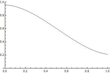
In order to see explicit examples of the function which is furthermore unimodular we could use this procedure (with different values for d)

z = True;
While[z,
  u = Random[];
  v = Random[];
  w = Random[];
  h[x_] = g[x] /. d -> 1.2 /. {f0 -> u, f1 -> v, ff1 -> -w};
  sh = Solve[h'[x] == 0, x];
  xx = x /. sh;
  z = xx \[Element] Reals && Not[xx[[1]] < 0 && xx[[2]] > 1]];
xx
h[x]
h'[1]
Plot[h[x], {x, 0, 1}, PlotRange -> {0, 1}]
(* 141203_Unimodular.jpg *)

(*

Out[904]= {-0.0203922, 1.05824}

Out[905]= 0.957347 - 0.0776871 x - 1.86812 x^2 + 1.2 x^3

Out[906]= -0.213927 *)

Best regards, Wolfgang