7
$\begingroup$

I have found NonlinearModelFit to be extremely useful in my work. Here I have fit 4 points to a function and am being asked to explain how the 95% SinglePredictionBands associated with the plot below were derived/computed. Can someone show how these bands can be computed from “first principles” ? In other words, I’d need to use Mathematica to independently produce the functions labeled lowerband and upperband. My code is below. Many thanks.

x = {1, 2, 3, 4};
y = {0.891, 0.885, 0.844, 0.836};
data1 = Transpose[{x, y}];
plot1 = ListPlot[data1, Frame -> True, 
FrameTicks -> {Range[0, 5, 1], Range[0.8, 0.9, .05], None, None}, 
FrameLabel -> {"X", "Y"}, PlotRange -> {{0, 5}, {0.8, 0.9}}, 
PlotStyle -> Red, ImageSize -> 500, 
LabelStyle -> Directive[Black, FontSize -> 14]];
Remove[a, b];
model1 = NonlinearModelFit[data1, a + b t^2, {a, b}, t] ;
Normal[model1];
params = model1["BestFitParameters"];
{a = params[[1, 2]], b = params[[2, 2]]};
predictionbands = model1["SinglePredictionBands"];
lower[t_] := predictionbands[[1]];
upper[t_] := predictionbands[[2]];
plot1a = Plot[model1[t], {t, 1, 4}, Frame -> True, PlotStyle -> Blue, 
PlotRange -> {{0, 4}, All}];
plot1b = Plot[model1[t], {t, 4, 9}, Frame -> True, 
PlotStyle -> {Blue, Dashed}, PlotRange -> All];
plot2a = Plot[lower[t], {t, 5, 9}, Frame -> True, 
FrameTicks -> {Range[0, 9, 1], Range[0, 0.9, .1], None, None},
PlotRange -> All, PlotStyle -> {Green, Dashed}];
plot2b = Plot[upper[t], {t, 5, 9}, Frame -> True, 
FrameTicks -> {Range[0, 9, 1], Range[0.5, 1, .1], None, None},
PlotRange -> {0.5, 1}, PlotStyle -> {Green, Dashed}];
text1 = Text["95% Upper Prediction Band", {7.5, .92}];
text2 = Text["95% Lower Prediction Band", {3.8, .68}];
text3 = Text["Nominal Prediction", {7, .75}];
plot3 = Show[plot1b, plot1a, plot2a, plot2b, plot1, 
AxesOrigin -> {0, 0}, PlotRange -> {.6, 1}, 
FrameTicks -> {Range[0, 9, 1], Range[.6, 1, .05], None, None}, 
FrameLabel -> {"X", "Y"}, 
Epilog -> {Line[{{-1, .65}, {9, .65}}], text1, text2, text3}, 
ImageSize -> 500, ImageSize -> 500, 
LabelStyle -> Directive[Black, FontSize -> 14]]
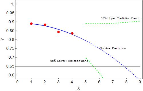
enter image description here

Here are the SinglePredictionBands that I need to independently produce.

lowerband = model1["SinglePredictionBands"][[1]]

0.894058 - 0.00400775 t^2 - 4.30265 Sqrt[0.000237726 - 0.0000163949 t^2 + 1.09299*10^-6 t^4]

upperband = model1["SinglePredictionBands"][[2]]

0.894058 - 0.00400775 t^2 + 4.30265 Sqrt[0.000237726 - 0.0000163949 t^2 + 1.09299*10^-6 t^4]

$\endgroup$
6

1 Answer 1

5
$\begingroup$

The fit given in this question, a + b t^2, is actually linear in a and b, so the regression line can be found with a linear fit, i.e.

x = {1, 2, 3, 4};
y = {0.891, 0.885, 0.844, 0.836};
data1 = Transpose[{x, y}];

n1 = Normal@NonlinearModelFit[data1, a + b t^2, {a, b}, t];

n2 = Normal@LinearModelFit[data1, {1, t^2}, t];

n1 == n2

True

The prediction intervals can be found using the two-variable least-squares model. First the data is linearised. Note this does not affect the regression coefficients:

data2 = Transpose[{x^2, y}];
n3 = Normal@LinearModelFit[data2, {1, s}, s]; 
CoefficientList[n2, t^2] == CoefficientList[n3, s]

True

Using the linearised data various quantities are computed:

MapIndexed[(X@#2 [[1]] = #1) &, x^2]; 
MapIndexed[(Y@#2 [[1]] = #1) &, y];

{n = Length[data2],
 ΣX = Sum[X[i], {i, n}],
 ΣY = Sum[Y[i], {i, n}],
 ΣXY = Sum[X[i] Y[i], {i, n}],
 ΣX2 = Sum[X[i]^2, {i, n}]}

{4, 30, 3.456, 25.403, 354}

{{a, b}} = {a, b} /. Solve[{
     (* Normal equations for straight line *)
     ΣY == n a + b ΣX,
     ΣXY == a ΣX + b ΣX2}, {a, b}];

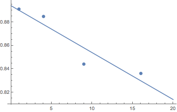
Show[Plot[a + b x, {x, 0, 20}], ListPlot[data2]]

enter image description here

(* Least-squares regression of Y on X *)
Array[(Yhat[#] = a + b X[#]) &, n];

Array[(e[#] = Y[#] - Yhat[#]) &, n];
(* Residual or unexplained sum of squares *)
RSS = Sum[e[i]^2, {i, n}];

(* Estimate of disturbance variance, s^2 *)
s2 = RSS/(n - 2);
s = Sqrt[s2];

Xmean = ΣX/n;
(* Derivation from sample x mean *)
Clear[x]; Array[(x[#] = X[#] - Xmean) &, n];
Σx2 = Sum[x[i]^2, {i, n}];

(* Confidence limit for +/-2 S.D. of the mean *)
σ = 2; cl = 2 (CDF[NormalDistribution[0, 1], σ] - 0.5)

0.9545

nvars = Length[{a, b}];
(* t-statistic *)
t = Quantile[StudentTDistribution[n - nvars], (1 + cl)/2]

4.52654

(* Estimated variance of a new observation *)
ev[X0_] := t s Sqrt[1 + 1/n + (X0 - Xmean)^2/Σx2]

interval[X0_] := {a + b X0 + ev[X0], a + b X0 - ev[X0]}

In accordance with the data linearisation the input to interval is squared.

lines[x_] := interval[x^2]

xvals = Table[i, {i, 5, 9, 0.04}];
{line1, line2} = Transpose[lines /@ xvals];

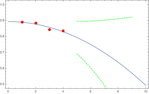
Show[Plot[a + b x^2, {x, 0, 10}], ListPlot[data1, PlotStyle -> Red],
 ListPlot[{Transpose[{xvals, line1}], Transpose[{xvals, line2}]},
  PlotStyle -> Directive[Green, Dashed],
  Joined -> True], AxesOrigin -> {0, 0}, ImageSize -> 480, 
 Frame -> True, PlotRange -> {{0, 10}, {0.5, 1}}]

enter image description here

The derivation of the estimated variance can be read in Econometric Methods (Ed.3) by J.Johnston, (chapter 2, The Two-Variable Linear Model), page 43.

$\endgroup$

Your Answer

By clicking “Post Your Answer”, you agree to our terms of service and acknowledge you have read our privacy policy.

Not the answer you're looking for? Browse other questions tagged or ask your own question.