3
$\begingroup$

The data is uploaded to Ideone http://ideone.com/ktIbVk , my code is :

data = ReadList["-10dBm.txt", {Number, Number}];
model = a/((b - f)/c)^2 + d;
result = NonlinearModelFit[data, model, {a, b, c, {d, 0}}, f];
result1 = result["ParameterTable"];
fitplot1 = plot[result[f], {f, 4.124, 4.133}];

the error is :

NonlinearModelFit::cvmit:
Failed to converge to the requested accuracy or precision within 100 iterations

Any ideas?

$\endgroup$
6
  • $\begingroup$ Increase the number of iterations? Look in the documentation: reference.wolfram.com/mathematica/ref/NonlinearModelFit.html $\endgroup$ Commented Jul 23, 2014 at 14:41
  • 1
    $\begingroup$ Add reasonable starting parameters for all parameters. $\endgroup$
    – Karsten7
    Commented Jul 23, 2014 at 14:44
  • $\begingroup$ Also, your model doesn't look like a Lorentzian? en.wikipedia.org/wiki/Spectral_line_shape#Line_shape_functions $\endgroup$ Commented Jul 23, 2014 at 15:00
  • $\begingroup$ My mistake, however the function model I chose is corrected. $\endgroup$
    – Hang Yang
    Commented Jul 23, 2014 at 15:16
  • $\begingroup$ So is it a Lorentzian, or isn't it? Because your function will be $=1/0$ at the point where f = b. My answer below is based on it being Lorentzian. $\endgroup$ Commented Jul 23, 2014 at 16:55

3 Answers 3

4
$\begingroup$

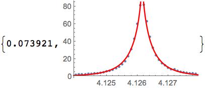
The timing for the plot from the answer from Alexei can be accelerated by using Evaluate and Prolog (or Epilog).

k = 0.725;

model = a*Exp[-Abs[(x - d)]^k/b];

ff = FindFit[data, {model, {a > 0, b > 0, 4.126 < d < 4.1262}},
    {{a, 80}, b, {d, 4.126}}, x] // Quiet;

xmin = Floor[Min[data[[All, 1]]], .001];
xmax = Ceiling[Max[data[[All, 1]]], .001];
ymax = Ceiling[Max[data[[All, 2]]], 5];

Show[{
   ListPlot[data],
   Plot[a*Exp[-Abs[(x - d)]^k/b] /. ff,
    {x, 4.12, 4.13},
    PlotStyle -> Red,
    PlotRange -> {{xmin, xmax}, {0, ymax}}]}] //
 Timing

enter image description here

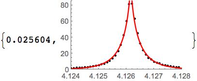
Timing using Evaluate to prevent repeated use of ReplaceAll

Show[{
   ListPlot[data],
   Plot[Evaluate[
     a*Exp[-Abs[(x - d)]^k/b] /. ff],
    {x, 4.12, 4.13},
    PlotStyle -> Red,
    PlotRange -> {{xmin, xmax}, {0, ymax}}]}] //
 Timing

enter image description here

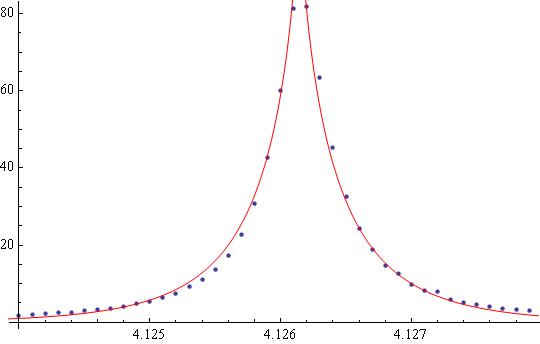
Timing using Prolog vice Show and ListPlot with Evaluate

Plot[Evaluate[
   a*Exp[-Abs[(x - d)]^k/b] /. ff],
  {x, 4.12, 4.13},
  Prolog -> Point[data],
  PlotStyle -> Red,
  PlotRange -> {{xmin, xmax}, {0, ymax}}] //
 Timing

enter image description here

While the difference is trivial in this case, for more complex functions the difference can be significant particularly if the plot is in a Manipulate.

$\endgroup$
1
  • 1
    $\begingroup$ @blochwave - does seem odd. I'll +1 yours to compensate somewhat. $\endgroup$
    – Bob Hanlon
    Commented Jul 23, 2014 at 20:27
9
$\begingroup$

Turns out I've got a bit of spare time, so here goes!

Following the information provided in the Wikipedia article on spectral lines, the model function you want for a Lorentzian is of the form:

$$ L=\frac{1}{1+x^{2}} $$

where

$$ x=\frac{A-x}{B} $$

with $A$ and $B$ as the position of the maximum, and twice the FWHM, respectively.

Now let's look at your model - notice the brackets around the parameter d - without it, the function is going to be $=1/0$ at the middle of the peak.

model = a/(((b - f)/c)^2 + d);
result = NonlinearModelFit[data, 
   model, {{a, 82.17435}, {b, 4.126155}, {c, 0.000283}, {d, 1.}}, f, 
   MaxIterations -> 500];
result["BestFitParameters"]
fitplot1 = 
 Show[ListPlot[data], 
  Plot[result[f], {f, 4.124, 4.133}, PlotRange -> Full]]

(* {a -> 86.104, b -> 4.12616, c -> 0.000276, d -> 1.05174} *)

And this result gives the following graph:
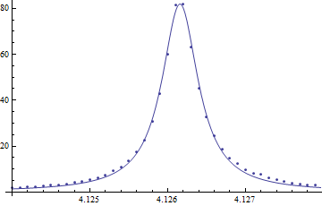
enter image description here

But what if I try it with different starting parameters?

model = a/(((b - f)/c)^2 + d);
result = NonlinearModelFit[data, 
  model, {{a, 82.}, {b, 4.126}, {c, 0.0002}, {d, 2.}}, f, 
  MaxIterations -> 500]
result["BestFitParameters"]
(* {a -> 123.998, b -> 4.12616, c -> 0.000230629, d -> 1.51461}*)

This still fits, but the parameters are all very different!

Heck, let's play around with the Method options of NonLinearModelFit.

I'll use Method->{NMinimize} here as per Methods for NonlinearModelFit, to perform a global optimization, with no initial guesses needed.

model = a/(((b - f)/c)^2 + d);
result = NonlinearModelFit[data, 
  model, {a, b, c, d}, f, 
  MaxIterations -> 500, Method -> {NMinimize}]
result["BestFitParameters"]
result["AdjustedRSquared"]
result["AIC"]
fitplot1 = 
 Show[ListPlot[data], 
  Plot[result[f], {f, 4.124, 4.133}, PlotRange -> Full]]

(* {a -> 6.14622, b -> 4.12616, c -> 0.00103591, d -> 0.0750752} *)
(* AdjustedRSquared = 0.997582 *)
(* AIC = 142.984 *)

Notice how the parameters are again different, but the result looks the same:

enter image description here

Now let's remove d from the equation and replace it with 1.

model = a/(((b - f)/c)^2 + 1.);
(* {a -> 81.8689, b -> 4.12616, c -> 0.000283838} *)
(* AdjustedRSquared = 0.997648 *)
(* AIC = 140.984 *)

Marginally better.


Also, let's put your data here rather than in a file.

data = {{4.124, 1.823}, {4.1241, 1.993}, {4.1242, 2.184}, {4.1243, 
   2.403}, {4.1244, 2.612}, {4.1245, 2.919}, {4.1246, 3.257}, {4.1247,
    3.637}, {4.1248, 4.133}, {4.1249, 4.76}, {4.125, 5.506}, {4.1251, 
   6.339}, {4.1252, 7.448}, {4.1253, 9.307}, {4.1254, 
   10.956}, {4.1255, 13.628}, {4.1256, 17.32}, {4.1257, 
   22.68}, {4.1258, 30.794}, {4.1259, 42.704}, {4.126, 
   59.972}, {4.1261, 81.436}, {4.1262, 81.723}, {4.1263, 
   63.309}, {4.1264, 45.292}, {4.1265, 32.623}, {4.1266, 
   24.327}, {4.1267, 18.823}, {4.1268, 14.627}, {4.1269, 
   12.612}, {4.127, 9.732}, {4.1271, 8.272}, {4.1272, 7.902}, {4.1273,
    6.021}, {4.1274, 5.232}, {4.1275, 4.523}, {4.1276, 
   4.023}, {4.1277, 3.602}, {4.1278, 3.212}, {4.1279, 3.025}}
$\endgroup$
2
  • 1
    $\begingroup$ My mistake.I just found it and got the right result. Your model function is right, and thanks for your examples. that is really helpful. $\endgroup$
    – Hang Yang
    Commented Jul 23, 2014 at 18:04
  • $\begingroup$ Glad I could help! If it worked for you, there's a little tick next to my answer for you to accept it, as per: mathematica.stackexchange.com/tour $\endgroup$ Commented Jul 23, 2014 at 18:05
3
$\begingroup$

Try this:

 k = 0.725;
model = a*Exp[-Abs[(x - d)]^k/b];
ff = FindFit[
  data, {model, {a > 0, b > 0, 4.126 < d < 4.1262}}, {{a, 80}, 
   b, {d, 4.126}}, x]
Show[{

  ListPlot[data],
  Plot[a*Exp[-Abs[(x - d)]^k/b] /. ff, {x, 4.12, 4.13}, 
   PlotStyle -> Red, PlotRange -> All]

  }]

It looks like the following:

enter image description here

$\endgroup$
3
  • $\begingroup$ Thank you! However, this model function is not what I want, the data is used to described a resonance phenomenon. $\endgroup$
    – Hang Yang
    Commented Jul 23, 2014 at 15:12
  • $\begingroup$ I used Excel to fit the data by using Minimum the difference between the fitted value and the data with "solver", it turned out that the parameter will have the best value "a=82.17436, b=4.126155, c=0.000283, d=0". However when I applied these value as the starting parameters, I could not get the best fit, the result is not right at all, why? $\endgroup$
    – Hang Yang
    Commented Jul 23, 2014 at 15:30
  • $\begingroup$ @Hang Yang First the answer to your first comment: I tried Lorenzian first. In particular, the same type of the model as in the answer of blochwave. It worked poor for me. I see from the answer above that there is a trick giving the solution. However, my experience of fitting shows that the necessity of tricks may mean that the data is poorly described by the model used, and another model should be looked for. That motivated the function I applied. The second question: I did not optimize the model. For example, why k=0.75? It is up to you, if you decide to use this model. $\endgroup$ Commented Jul 24, 2014 at 7:11

Your Answer

By clicking “Post Your Answer”, you agree to our terms of service and acknowledge you have read our privacy policy.

Not the answer you're looking for? Browse other questions tagged or ask your own question.