How can I speed up this code？

Question

There are 4 variables in this multiple sum, and only 2 are used. This question has the similar scenario as the previous one How can I speed up this code with multiple sum？, but the calculation process is different. This code takes about 1 min 38 sec to obtain the results, but I hope the time can be shortened to several seconds. Any help or suggestion will be highly appreciated!

the code is bellow :

data = Table[Exp[-((i + j - 50.)/5)^2] Exp[-((i - j)/5)^2], {i, 50}, {j, 50}];
data = Chop[data, 0.00001];
data = data/Sqrt[Sum[(data[[i, j]])^2, {i, 1, 50}, {j, 1, 50}]];
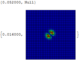
ListDensityPlot[data, InterpolationOrder -> 0, Mesh -> All,  PlotRange -> All, ColorFunction -> (Blend[{Hue[2/3], Hue[0]}, #] &)]


S1[i_, j_, k_, m_, t_] := (data[[i, k]] data[[j, m]])^2 + (data[[j, k]] data[[i, 
  m]])^2 - 2 data[[i, k]] data[[j, m]] data[[j, k]] data[[i, 
 m]] Cos[(2 \[Pi]*(3*10^8)/(1584 - 5 + j*0.1 - 0.05) - 
    2 \[Pi]*(3*10^8)/(1584 - 5 + i*0.1 - 0.05)) t];
S2[i_, j_, t_] := 1/4*\!\(\*UnderoverscriptBox[\(\[Sum]\), \(k = 1\), \(50\)]\(\*UnderoverscriptBox[\(\[Sum]\), \(m = 1\), \(50\)]S1[i, j, k, m, 
  t]\)\);
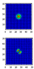
data2 = Table[S2[i, j, 4*0.001], {i, 1, 50}, {j, 1, 50}];
ListDensityPlot[data2, InterpolationOrder -> 0, Mesh -> All, PlotRange -> All, ColorFunction -> (Blend[{Hue[2/3], Hue[0]}, #] &)]

Answer 1

You should have read Simon Woods's answer more carefully. The difference between this question and the previous one is just you don't need to sum over $j$ and $k$ now, with almost same analysis, you can figure out that data2 is equal to

$$ 2 {\left((d.d^T)^2\right)}_{ij}(1 - f_{ij})/4$$

So here is the code:

a = AbsoluteTiming;
data0 = Table[Exp[-((i + j - 50.)/5)^2] Exp[-((i - j)/5)^2], {i, 50}, {j, 50}];
data = Partition[Normalize@Flatten@Chop[data0, 0.00001], 50]; // a
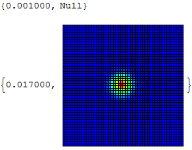
ArrayPlot[data, Mesh -> All, MeshStyle -> Black, 
                ColorFunction -> (Blend[{Hue[2/3], Hue[0]}, #] &)] // a

Notice my modification for data. (As mentioned by Simon in the previous post, you will generally get much better performance by acting on a whole array at once instead of on each element individually.) Also, I chose ArrayPlot instead of ListDensityPlot because it's faster and has the same effect as your ListDensityPlot with the option InterpolatingOrder -> 0.

The rest part is nearly the same as Simon's:

f[i_, j_, t_] = Cos[(2 Pi (3 10^8)/(1584 - 5 + 0.1 j - 0.05) - 
                2 Pi (3 10^8)/(1584 - 5 + 0.1 i - 0.05)) t];
data2 = 2 (data.Transpose[data])^2 (1 - Array[f[##, 4 0.001] &, {50, 50}]) / 4; // a
ArrayPlot[data2, Mesh -> All, MeshStyle -> Black, 
                 ColorFunction -> (Blend[{Hue[2/3], Hue[0]}, #1] &)] // a

Answer 2

Like Ajasja said in a comment, Compile is your best friend here (short of completely rewriting S1 and S2 like in your other question). Simply compiling everything together:

With[{d = data},
  S2 = Compile[
    {{i, _Integer}, {j, _Integer}, {t, _Real}},
     1/4*Sum[
      (d[[i, k]] d[[j, m]])^2 
       + (d[[j, k]] d[[i, m]])^2 
       - 2 d[[i, k]] d[[j, m]] d[[j, k]] d[[i, m]] Cos[
         (2 \[Pi]*(3*10^8)/(1584 - 5 + j*0.1 - 0.05) - 
            2 \[Pi]*(3*10^8)/(1584 - 5 + i*0.1 - 0.05)) t
         ],
      {k, 1, 50}, {m, 1, 50}
      ],
    CompilationTarget -> "C", RuntimeOptions -> "Speed"
    ]
  ];

gives a considerably speed increase:

(data2 = Table[S2[i, j, 4*0.001], {i, 1, 50}, {j, 1, 50}];) // Timing

{0.915097, Null}

Note that inserting data into the compiled function with With is key to getting a big speed increase. My guess is that the compiled function then doesn't have to go to the main evaluation loop to acces data each time, which would severely slow performance.