You should have read Simon Woods's answerSimon Woods's answer more carefully. The difference between this question and the previous one is just you don't need to sum over $j$ and $k$ now, with almost same analysis, you can figure out that data2 is equal to
$$ 2 {\left((d.d^T)^2\right)}_{ij}(1 - f_{ij})/4$$
So here is the code:
a = AbsoluteTiming;
data0 = Table[Exp[-((i + j - 50.)/5)^2] Exp[-((i - j)/5)^2], {i, 50}, {j, 50}];
data = Partition[Normalize@Flatten@Chop[data0, 0.00001], 50]; // a
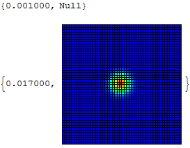
ArrayPlot[data, Mesh -> All, MeshStyle -> Black,
                ColorFunction -> (Blend[{Hue[2/3], Hue[0]}, #] &)] // a

Notice my modification for data. (As mentioned by Simon in the previous post, you will generally get much better performance by acting on a whole array at once instead of on each element individually.) Also, I chose ArrayPlot instead of ListDensityPlot because it's faster and has the same effect as your ListDensityPlot with the option InterpolatingOrder -> 0.
The rest part is nearly the same as Simon's:
f[i_, j_, t_] = Cos[(2 Pi (3 10^8)/(1584 - 5 + 0.1 j - 0.05) -
                2 Pi (3 10^8)/(1584 - 5 + 0.1 i - 0.05)) t];
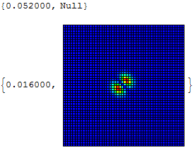
data2 = 2 (data.Transpose[data])^2 (1 - Array[f[##, 4 0.001] &, {50, 50}]) / 4; // a
ArrayPlot[data2, Mesh -> All, MeshStyle -> Black,
                 ColorFunction -> (Blend[{Hue[2/3], Hue[0]}, #1] &)] // a

