7
$\begingroup$

I want to write a computer program to generate 3-D plots (with x-y-t axes) to demonstrate the evolution of the two missiles in the following case:

i. $x = 100t$, $y = 80t-16t^2$ for $0\leq t\leq 5$ for the incoming missile

ii. $x= 500-200(t-2)$, $y = 80(t-2)-16(t-2)^2$ for $2\leq t\leq 7$ for the interceptor missile

I coded it like this:

ParametricPlot3D[{{100 t, 80 t - 16 t^2, 60 t}, {500 - 200 (s - 2), 
80 (s - 2) - 16 (s - 2)^2, s}}, {t, 0, 5}, {s, 2, 7}]

The problem is that How can I animate this two functions in 3D form (with x-y-t axes)? I want it to display two moving objects,so i can see if there's any collision.By the way,please help me to correct the code if I'm wrong.

$\endgroup$

3 Answers 3

13
$\begingroup$

Maybe you want an animation parameterized by the time $t$? This would do it in an interactive way:

With[{missileSize = 10},
 Manipulate[
  Graphics[{
    {Red,
     Disk[
      {100 t, 80 t - 16 t^2}, missileSize
      ]},
    {Blue,
     Disk[
      {500 - 200 (t - 2), 80 (t - 2) - 16 (t - 2)^2}, missileSize
      ]}
    },
   Frame -> True,
   GridLines -> Automatic,
   PlotRange -> {{0, 800}, {-200, 400}},
   AspectRatio -> Automatic],
  {t, 0, 7}]
 ]

Alternatively, you could create an animation like this:

t = Table[Graphics[{
     {Red,
      Disk[
       {100 t, 80 t - 16 t^2}, 10
       ]},
     {Blue,
      Disk[
       {500 - 200 (t - 2), 80 (t - 2) - 16 (t - 2)^2}, 10
       ]}
     },
    Frame -> True,
    PlotRange -> {{0, 800}, {-200, 400}},
    AspectRatio -> Automatic],
   {t, 0, 5, .1}];

ListAnimate[t]
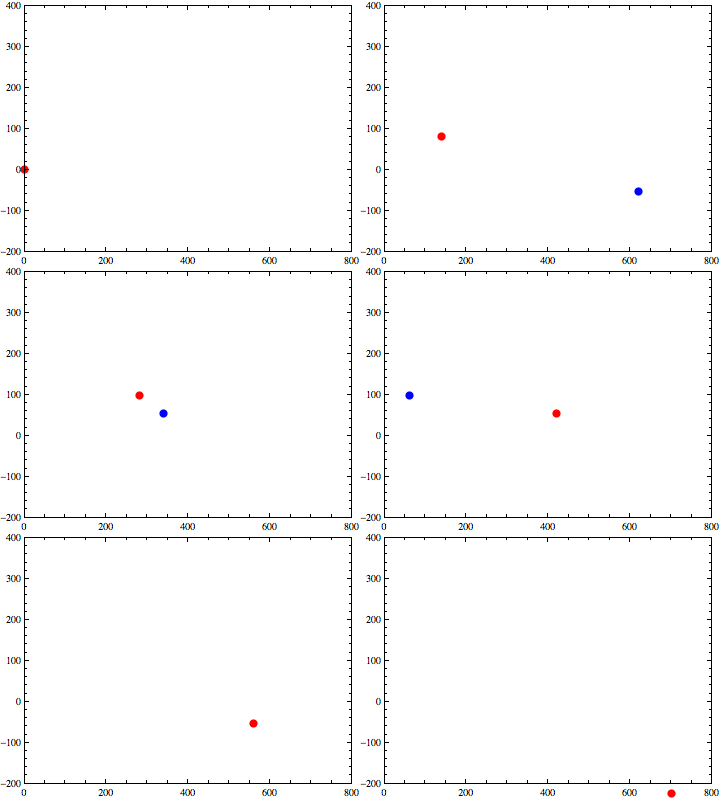
missile animation

The animation above was created with

Export["missiles.gif", t]

Edit

Since it was asked in the comment, I'll add the 3D analogue here, too - although Verbeia already did something like it with Manipulate:

xMin = 0;
xMax = 800;
yMin = -200;
yMax = 200;
zMin = -200;
zMax = 400;
ground = {Green, 
   Polygon[{{xMin, yMin, zMin}, {xMin, yMax, zMin}, {xMax, yMax, 
      zMin}, {xMax, yMin, zMin}}]};

t = Table[
   Graphics3D[{ground, {Red, 
      Sphere[{100 t, 0, 80 t - 16 t^2}, 10]}, {Blue, 
      Sphere[{500 - 200 (t - 2), 0, 80 (t - 2) - 16 (t - 2)^2}, 10]}},
     Boxed -> True, 
    PlotRange -> {{xMin, xMax}, {yMin, yMax}, {zMin, zMax}}], {t, 0, 
    6, .1}];

ListAnimate[t]
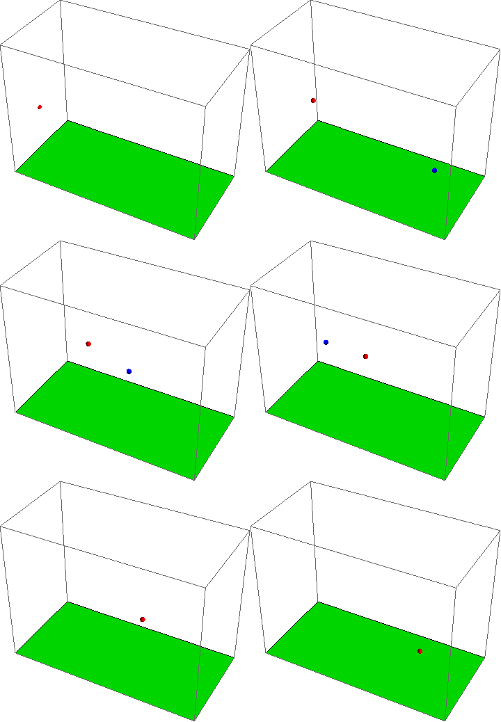
bullets in 3d

If you compare to the 2D code, I just replaced Disk by Sphere, made the height the z coordinate and set the y coordinate of the projectiles to 0.

The other changes are just small tweaks: I defined the plot range as variables so I can use them to define a rectangular Polygon representing the ground. Instead of the Framed option, there is the Boxed option (which can also be omitted or set to False).

$\endgroup$
1
  • $\begingroup$ thank you for your answer,it's pretty clear and understandable. but how can i plot it in 3D form?I have tried using Graphic3D@Sphere as in Verbeia's answer, but i couldnt make it. $\endgroup$
    – mckareem
    Commented May 4, 2012 at 11:12
9
$\begingroup$

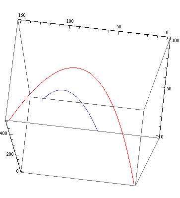
What you could do with ParametricPlot3D is to observe the trajectories in the $\{x,y,t\}$ space:

Show[
 ParametricPlot3D[{30 t, 100 t, 80 t - 16 t^2}, {t, 0, 5}, PlotStyle -> Red],
 ParametricPlot3D[{30 t, (500 - 200 ( t - 2)),  80 (t - 2) - 16 (t - 2)^2}, {t, 2, 7}]]

enter image description here

(the $t$ coordinate has been dilated to get a better aspect ratio)

$\endgroup$
8
$\begingroup$

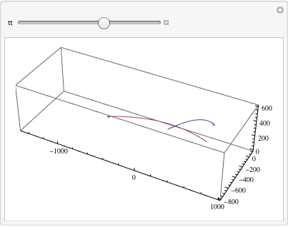
This version combines the Manipulate approach suggested by Jens with the ParametricPlot3D approach used by belisarius, to get a version with flying "cannonballs" made out of Sphere primitives, as well as their trajectories to that point (tt), plotted using ParametricPlot3D.

Manipulate[
 Show[{ParametricPlot3D[{{100 t, 80 t - 16 t^2, 60 t}, {500 - 200 t, 
      80 t - 16 t^2, t + 2}}, {t, 0, tt}, PlotRangePadding -> 20, 
    PlotRange -> {{-1500, 1000}, {-800, 100}, {0, 600}}], 
   Graphics3D@Sphere[{100 tt, 80 tt - 16 tt^2, 60 tt}, 15], 
   Graphics3D@Sphere[{500 - 200 tt, 80 tt - 16 tt^2, tt + 2}, 15]}], 
 {tt, 0.1, 10}]

The explicit PlotRange stops the box resizing. I included the PlotRangePadding option so that the cannonballs don't get cut off at the edge of the plot.

enter image description here

belisarius has pointed out to me that you can avoid working out the total plot range using a “hidden graph” technique.

Manipulate[ 
Show[{ParametricPlot3D[{{100 t, 80 t - 16 t^2, 60 t}, 
  {500 - 200 t, 80 t - 16 t^2, t + 2}}, {t, 0, 10}, 
  PlotRangePadding -> Scaled[0.2], PlotStyle -> None], 
 ParametricPlot3D[{{100 t, 80 t - 16 t^2, 60 t}, 
  {500 - 200 t, 80 t - 16 t^2, t + 2}}, {t, 0, tt}, 
 PlotRangePadding -> Scaled[0.2]], 
 Graphics3D@Sphere[{100 tt, 80 tt - 16 tt^2, 60 tt}, 55], 
 Graphics3D@Sphere[{500 - 200 tt, 80 tt - 16 tt^2, tt + 2}, 55]}], 
{tt, 0.1, 10}]

To be honest I would never have expected these trajectories to meet because the following yields an empty list (no solutions).

Solve[Thread[{100 t, 80 t - 16 t^2, 60 t} == {500 - 200 (t), 
    80 (t) - 16 (t)^2, t + 2}], t]
$\endgroup$
1
  • 1
    $\begingroup$ I had thought of using the space shuttle example data for this... but decided that would be too macabre. $\endgroup$
    – Jens
    Commented Apr 30, 2012 at 5:02

Your Answer

By clicking “Post Your Answer”, you agree to our terms of service and acknowledge you have read our privacy policy.

Not the answer you're looking for? Browse other questions tagged or ask your own question.