2
$\begingroup$

I have a following systeme :

\begin{equation} \left\{ \begin{array}{rcr} (\beta+\frac{1}{2}\delta^{2})\nu_{1}(u)-\delta\nu_{2}(u)+\nu_{3}(u)& = &0\\ (\beta+\frac{1}{2}\delta^{2})\upsilon_{1}(u)-\delta\upsilon_{2}(u)+\upsilon_{3}(u)& < &0\\ \end{array} \right. \end{equation}

where

\begin{align*} &\nu_{1}(u)= q(u)f[q(u)],\\ &\nu_{2}(u)= f[q(u)]^2 + F(x)q(u)f[q(u)],\\ &\nu_{3}(u)= \left(u (f[q(u)])^2 + \frac{1}{2}u^2q(u)f[q(u)]\right),\\ &q[u] := Quantile[NormalDistribution[0, 1], u], \ (the \ quantale \ at \ u)\\ &f[q(u)]=PDF[NormalDistribution[0, 1], q(u)] \ (the \ density \ at \ q(u)), \end{align*}

and for the inequality, $\upsilon_{i}(u)=\nu_{i}^\prime(u)$ with respect $q(u)$ for $ i\in \{1,2,3\}$ with $(\beta,\delta,u)\in [0.1]\times[0.1]\times[0.1]$.

I would like to look at the projection of this system of equation onto the plane $(\beta,\delta)$ and $(u,\delta)$ in Mathematica or in r.

My code sets up the full 3-d view of the 3D plot, which is not what I want. And I think there are some thing wrong in my picture. I'd like to see two of the views $(\beta,\delta)$ and $(u,\delta)$ on different figure.

q[u_] := Quantile[NormalDistribution[0, 1], u]
f[x_] := PDF[NormalDistribution[0, 1], x]
h1[u_, a_, e_] := ((((a^2)/2 + e)*(-q[u])*(f[q[u]])) - 
a*(-q[u]*f[q[u]]*u  +   f[q[u]]^2) + 
u*f[q[u]]^2 - (u^2)/2*q[u]*f[q[u]])/(1/6 - a/2 + (a^2)/2 + e)
h2[u_, a_, e_] := (((a^2)/2 + e)*((q[u]^2) - 1)*f[q[u]]) - 
a*(u*(q[u]^2 - 1)*f[q[u]] - 3* q[u]*  f[q[u]]^2) + f[q[u]]^3 - 
2*u*q[u]*f[q[u]]^2 - 
u*q[u]*f[q[u]]^2 + ((u^2)/2)*(q[u]^2 - 1)*f[q[u]]
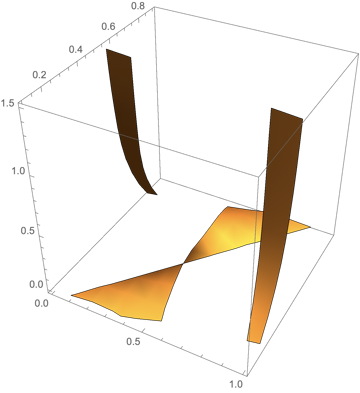
ContourPlot3D[ h1[u, a, e] == 0, 
{a, 0, 1}, {u, 0.1, 0.9}, {e, 0, 1.5}, 
RegionFunction -> Function[{u, a, e}, h2[u, a, e] > 0]]

The graph 3D : enter image description here
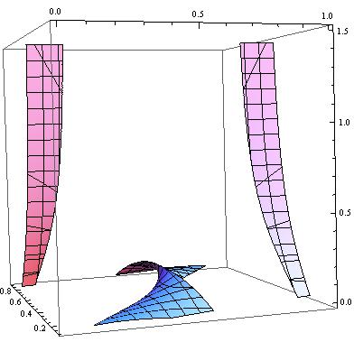
I want to try do verify if my plot 3D is true and if it is possible to have the projection on both plan $(\beta,\delta)$ and $(u,\delta)$.

Any thoughts on the best way to do this?

$\endgroup$
6
  • $\begingroup$ As I understood, projections are solutions of an initial system with one of coordinates is equal to zero. So, (Beta, Delta) view appears as when u=0. And it could be drawn in usual ContourPlot Additionally, you can see projections at your 3D graph just using appropriate ViewPoint $\endgroup$
    – Rom38
    Commented May 19, 2014 at 22:34
  • $\begingroup$ No the projection is all the image of the curve on the surface (Beta, Delta) , for example if we consider a sphere x^2+y^2+z^2=0 this is the equation of the sphere, and the projection on (y,z) is a circle. I want to do the same here. $\endgroup$
    – Lea
    Commented May 19, 2014 at 22:51
  • $\begingroup$ Aha :) So, ViewPoint helps you to see it $\endgroup$
    – Rom38
    Commented May 19, 2014 at 23:09
  • $\begingroup$ Your expression contains a bracket mismatch. Could you please check? $\endgroup$
    – Yves Klett
    Commented May 20, 2014 at 8:48
  • 1
    $\begingroup$ This takes ages to evaluate so it would be handy if you included a simple example. I think this, this and this are heavily related if not duplicates $\endgroup$
    – gpap
    Commented May 20, 2014 at 11:09

3 Answers 3

5
$\begingroup$

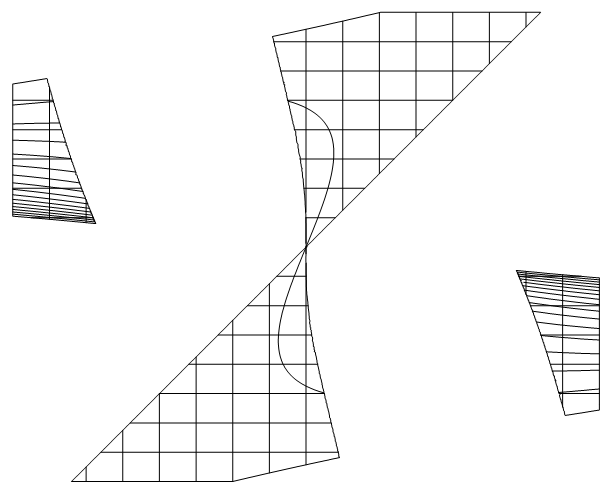
This may serve as a starting point - extract all Lines from the 3D graphics and get rid of the third component in all coordinate triples (an old but useful trick):

plot = ContourPlot3D[
   h1[u, a, e] == 0, {a, 0, 1}, {u, 0.1, 0.9}, {e, 0, 1.5}, 
   RegionFunction -> Function[{u, a, e}, h2[u, a, e] > 0]];

Cases[plot[[1]] // Normal, _Line, 
   Infinity] /. {x_?NumericQ, y_?NumericQ, z_?NumericQ} :> {x,y} // Graphics

Mathematica graphics

$\endgroup$
2
  • $\begingroup$ Damn you and your quick typing! $\endgroup$
    – gpap
    Commented May 20, 2014 at 11:13
  • $\begingroup$ @gpap meet me at noon here :D $\endgroup$
    – Yves Klett
    Commented May 20, 2014 at 12:14
2
$\begingroup$

I guess, the best way to draw projections is select the resulting 3D-graphics and to choose viewpoint when styling menu appeared. For orthogonal projections it should be ViewPoint -> {0, \[Infinity], 0} ViewPoint -> {\[Infinity], 0, 0} ViewPoint -> {0, 0, \[Infinity]}

$\endgroup$
0
$\begingroup$

Try this:

q[u_] := Quantile[NormalDistribution[0, 1], u]
f[x_] := PDF[NormalDistribution[0, 1], x]
h1[u_, a_, 
  x_] := ((((a^2)/2 + x)*(-q[u])*(f[q[u]])) - 
    a*(-q[u]*f[q[u]]*u + f[q[u]]^2) + 
    u*f[q[u]]^2 - (u^2)/2*q[u]*f[q[u]])/(1/6 - a/2 + (a^2)/2 + x)
h2[u_, a_, x_] := (((a^2)/2 + x)*((q[u]^2) - 1)*f[q[u]]) - 
  a*(u*(q[u]^2 - 1)*f[q[u]] - 3*q[u]*f[q[u]]^2) + f[q[u]]^3 - 
  2*u*q[u]*f[q[u]]^2 - 
  u*q[u]*f[q[u]]^2 + ((u^2)/2)*(q[u]^2 - 1)*f[q[u]]
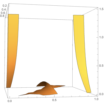
ContourPlot3D[h1[u, a, x] == 0, {a, 0, 1}, {u, 0.1, 0.9}, {x, 0, 1.5},
  RegionFunction -> Function[{u, a, x}, h2[u, a, x] > 0], 
 PerformanceGoal -> "Speed"]

Graphics3D

Second perspective

PerformanceGoal is a Mathematica built-in. It can be set to Speed and or Quality. Speed is the option of the trick to be fast.

The output looks brilliant and close to the long time calculation. I did it with V12.0.

Cases[%443[[1]] // Normal, _Line, 
   Infinity] /. {x_?NumericQ, y_?NumericQ, z_?NumericQ} :> {x, 
    y} // Graphics

Graphics

is already close to the other solution and a fast calculation too.

This runs in seconds than in hours.

The time-consuming parameter is Mesh. For Mesh -> 10 the plane results take a two-minutes effort and:

Grapics result with 10 mesh lines

The PerformanceGoal compiles internally the distributions functions and uses only a polynomial interpolated approximation. That results in the speed up.

$\endgroup$

Your Answer

By clicking “Post Your Answer”, you agree to our terms of service and acknowledge you have read our privacy policy.

Not the answer you're looking for? Browse other questions tagged or ask your own question.