Minimizing a function of many coordinates

Question

I'm trying to obtain a series of points on the unit sphere with a somewhat homogeneous distribution, by minimizing a function depending on distances (I took $\exp(-d)$). My points are represented by spherical angles $\theta$ and $\phi$, starting by choosing equidistributed random vectors:

pts = Apply[{2 π #1, ArcCos[2 #2 - 1]} &, RandomReal[1, {100, 2}], 1];

The energy function is defined first:

energy[p_] := Module[{cart},
  cart = Apply[{Sin[#1]*Cos[#2], Sin[#1]*Sin[#2], Cos[#1]} &, p, 1];
  Total[Outer[Exp[-Norm[#1 - #2]] &, cart, cart, 1], 2]
]

But now, I can’t manage to get the right routine for minimization. I tried FindMinimum, which does local minimization from a given starting point, which is what I want. But it should operate on an expression of literal variables, so I'm kind of screwed:

FindMinimum[energy[p], {p, pts}]

 

Outer::normal: Nonatomic expression expected at position 2 in Outer[Exp[-Norm[#1-Slot[<<1>>]]]&,p,p,1]. >>
FindMinimum::nrnum: The function value […] is not a real number at {p} = […] >>

The above obviously doesn't work, but I don't think it's wise to introduce a series of 200 literal variables. There has to be another way, hasn't it? Or is there an efficient way of introducing a lot of variables?

Answer 1

To get arbitrarily many formal variables, you can use Array. But with those variables, your function definition won't work because of the Apply statement. So I modified your definition as follows (I reduced the point number for testing purposes):

pts = Apply[{ArcCos[2 #2 - 1], 2 \[Pi] #1} &, RandomReal[1, {10, 2}], 1];
Clear[energy];
Clear[a];
vars = Array[a, {Length[pts], 2}];
energy[p_] := 
  Module[{cart}, 
   cart = Map[{Sin[#[[1]]]*Cos[#[[2]]], Sin[#[[1]]]*Sin[#[[2]]], 
       Cos[#[[1]]]} &, p];
   Total[Outer[Exp[-Norm[#1 - #2]] &, cart, cart, 1], 2]];
FindMinimum[energy[vars], Transpose[{Flatten@vars, Flatten@pts}]]

{32.2548, {a[1, 1] -> 1.93787, a[1, 2] -> 1.72361, a[2, 1] -> 1.11355, a[2, 2] -> 0.893035, a[3, 1] -> 6.21077, a[3, 2] -> 2.1405, a[4, 1] -> 3.06917, a[4, 2] -> 2.14062, a[5, 1] -> 1.06997, a[5, 2] -> 2.50937, a[6, 1] -> 4.21367, a[6, 2] -> 1.69561, a[7, 1] -> 5.07748, a[7, 2] -> 2.48594, a[8, 1] -> 4.31041, a[8, 2] -> 0.111206, a[9, 1] -> 4.25016, a[9, 2] -> 3.31368, a[10, 1] -> 5.11923, a[10, 2] -> 0.955784}}

The form of the array passed to energy matches the $N\times2$ dimension list that is expected by the line creating the cart variable. In the FindMinimum statement the dummy variables and initial conditions are specified as a single list of pairs by using Flatten on both.

There is the usual wrinkle that the minimization may need to be tweaked for precision, but that's a different issue.

Finally, to get the minimizing point list, you have to do

vars/.Last[%]

Edit

Depending on the function to be optimized, it's sometimes faster to avoid the use of derivatives by specifying the initial conditions for FindMinimum in the form of three numbers:

FindMinimum[energy[vars], 
Transpose[{Flatten@vars, Flatten@pts, Flatten@pts - .1, Flatten@pts + .1}]]

Edit 2

I did get a significant speed-up with this for your example, but the performance depends on the random starting points (and on the choice of bracket width) so I can't say anything definitive. That seems like a topic for a different question.

Edit 3

Though I didn't look at the speed issue in detail, forcing FindMinimum to work with numerical derivatives may be the worst option here. That will happen if you define your function energy only for numerical arguments, as in

energy[p : {{_?NumericQ, _?NumericQ} ..}] := 

followed by either your own or my initial definition above. So although that's a common advice people give in these applications, it is not going to be the fastest approach here.

Edit 4

I just had another idea on how to improve the speed of my solution: the use of Norm might make it harder to estimate the Hessian for this function. And indeed, when I got rid of Norm there was a significant speed gain (note that the initial solution above is already faster than the _?NumericQ approach even when the latter is compiled while mine is not). I think this is worth adding here because Norm seems like a natural thing to use in pair potentials, even if the energy expression becomes more complicated than the one in this question.

So here is the new version, with Norm replaced by Sqrt[(#1 - #2).(#1 - #2)]. Observe that I have now put back the original particle number of 100 because on my laptop this takes less than 8 seconds to evaluate!

pts = Apply[{ArcCos[2 #2 - 1], 2 \[Pi] #1} &, RandomReal[1, {100, 2}], 1];
Clear[energy];
Clear[a];
vars = Array[a, {Length[pts], 2}];
energy[p_] := 
  Module[{cart}, 
   cart = Map[{Sin[#[[1]]]*Cos[#[[2]]], Sin[#[[1]]]*Sin[#[[2]]], 
       Cos[#[[1]]]} &, p];
   Total[Outer[Exp[-Sqrt[(#1 - #2).(#1 - #2)]] &, cart, cart, 1], 2]];
FindMinimum[energy[vars], Transpose[{Flatten@vars, Flatten@pts}]]

Oh, and one more thing I changed (unrelated to the question), is to switch your definitions of polar and azimuthal angles in pts.

Answer 2

I played around with a few plausible variants on the energy. In all cases I compared the result using the original energy function. Some things I learned:

(1) Some variants will tend to give results that do quite well when gauged via the original energy.

(2) Others (not shown below) will do poorly because they weigh the far values too heavily. This, alas, means we cannot easily use the GaussNewton (LevenbergMarquardt) method, since it is the operations of squaring that hurts us. Well, maybe there are ways around this.

(3) Summing over only distinct pairs rather than all pairs cuts the time in half. I will speculate that the bulk of time is spent in evaluating derivatives and not in the function evaluations themselves, as I am fairly certain Total[Outer[...]] will beat Sum even when the latter only need account for half or so as many pairs.

(4) For one energy variant I got a modest speed improvement using the ConjugateGradient method.

(5) Scaling appears to be quadratic in the number of points (no huge surprise, I guess).

(6) We can handle 200 points in 24 seconds on my desktop machine.

In[254]:= 
pts = Apply[{ArcCos[2 #2 - 1], 2 \[Pi] #1} &, RandomReal[1, {100, 2}],
    1];
Clear[a];
vars = Array[a, {Length[pts], 2}];

Here is the basic case.

In[292]:= 
energy[p_] := 
  Module[{cart}, 
   cart = Map[{Sin[#[[1]]]*Cos[#[[2]]], Sin[#[[1]]]*Sin[#[[2]]], 
       Cos[#[[1]]]} &, p];
   Total[Outer[Exp[-Sqrt[(#1 - #2).(#1 - #2)]] &, cart, cart, 1], 2]];

In[293]:= 
t = Timing[{min, vals} = 
     Quiet[FindMinimum[energy[vars], 
       Transpose[{Flatten@vars, Flatten@pts}], 
       MaxIterations -> 1000]];];
{t, min}

Out[294]= {{14.1, Null}, 2978.01}

We use Sum over distinct pairs from here onward.

In[295]:= 
energy2[p_] := 
  Module[{cart}, 
   cart = Map[{Sin[#[[1]]]*Cos[#[[2]]], Sin[#[[1]]]*Sin[#[[2]]], 
       Cos[#[[1]]]} &, p];
   Sum[Exp[-Sqrt[(cart[[j]] - cart[[k]]).(cart[[j]] - 
          cart[[k]])]], {j, Length[p] - 1}, {k, j + 1, Length[p]}]];

In[296]:= 
t2 = Timing[{min2, vals2} = 
     Quiet[FindMinimum[energy2[vars], 
       Transpose[{Flatten@vars, Flatten@pts}], 
       MaxIterations -> 1000]];];
{t2, min2, energy[vars /. vals2]}

Out[297]= {{6.58, Null}, 1439., 2978.01}

Minimize the sum of reciprocals of the pairwise distances squared.

In[298]:= energy3[p_] := Module[{cart},
  cart = Map[{Sin[#[[1]]]*Cos[#[[2]]], Sin[#[[1]]]*Sin[#[[2]]], 
      Cos[#[[1]]]} &, p];
  Sum[1/((cart[[j]] - cart[[k]]).(cart[[j]] - cart[[k]])), {j, 
    Length[p] - 1}, {k, j + 1, Length[p]}]
  ]

In[299]:= 
t3 = Timing[{min3, vals3} = 
     Quiet[FindMinimum[energy2[vars], 
       Transpose[{Flatten@vars, Flatten@pts}],
       MaxIterations -> 1000]];];
{t3, min3, energy[vars /. vals3]}

Out[300]= {{6.72, Null}, 1439., 2978.01}

This variant on energy happened to get a bit faster using a nondefault method setting.

In[301]:= 
t3b = Timing[{min3b, vals3b} = 
     Quiet[FindMinimum[energy3[vars], 
       Transpose[{Flatten@vars, Flatten@pts}], MaxIterations -> 1000, 
       Method -> "ConjugateGradient"]];];
{t3b, min3b, energy[vars /. vals3b]}

Out[302]= {{5.23, Null}, 5340.65, 2978.01}

Maximize sum of distances. I will mention that using the sum of squares, which i would prefer to do, fails to give a useful result. It puts half the points one place and the other half at the polar opposite, I believe. That comes from the further distances getting relatively more weight in the objective function.

In[304]:= energy4[p_] := Module[{cart},
  cart = Map[{Sin[#[[1]]]*Cos[#[[2]]], Sin[#[[1]]]*Sin[#[[2]]], 
      Cos[#[[1]]]} &, p];
  Sum[Sqrt[((cart[[j]] - cart[[k]]).(cart[[j]] - cart[[k]]))], {j, 
    Length[p] - 1}, {k, j + 1, Length[p]}]
  ]

In[305]:= 
t4 = Timing[{min4, vals4} = 
     Quiet[FindMaximum[energy4[vars], 
       Transpose[{Flatten@vars, Flatten@pts}], 
       MaxIterations -> 1000]];];
{t4, min4, energy[vars /. vals4]}

Out[306]= {{8.44, Null}, 6662.64, 2978.}

Similar to a couple of tries above, but with distances instead of squared distances.

In[308]:= energy5[p_] := Module[{cart},
  cart = Map[{Sin[#[[1]]]*Cos[#[[2]]], Sin[#[[1]]]*Sin[#[[2]]], 
      Cos[#[[1]]]} &, p];
  Sum[1/((cart[[j]] - cart[[k]]).(cart[[j]] - cart[[k]]))^(1/2), {j, 
    Length[p] - 1}, {k, j + 1, Length[p]}]
  ]

In[309]:= 
t5 = Timing[{min5, vals5} = 
     Quiet[FindMinimum[energy5[vars], 
       Transpose[{Flatten@vars, Flatten@pts}], 
       MaxIterations -> 1000]];];
{t5, min5, energy[vars /. vals5]}

Out[310]= {{6.04, Null}, 4448.45, 2978.01}

Notice that all of these agreed fairly closely to six places in terms of the original energy function.

Now we'll go to 200 points and use the fastest variant from above.

In[319]:= 
pts200 = Apply[{ArcCos[2 #2 - 1], 2 \[Pi] #1} &, 
   RandomReal[1, {200, 2}], 1];
vars200 = Array[a, {Length[pts200], 2}];
t200 = Timing[{min200, vals200} = 
     Quiet[FindMinimum[energy3[vars200], 
       Transpose[{Flatten@vars200, Flatten@pts200}],
       MaxIterations -> 1000,
       Method -> "ConjugateGradient"]];];
{t200, min200, energy[vars200 /. vals200]}

Out[322]= {{23.59, Null}, 24816.3, 11891.3}

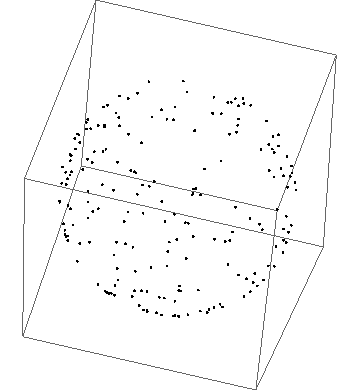
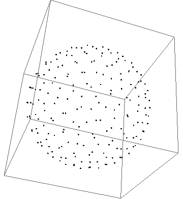
Here I crib Mark McClure's code to show both the original points and the result of the optimization. The pictures will have to speak for themselves because i'm not going to speak for them.

In[323]:= 
pts3D = {Sin[#[[1]]]*Cos[#[[2]]], Sin[#[[1]]]*Sin[#[[2]]], 
     Cos[#[[1]]]} & /@ pts200;
Graphics3D[Point[pts3D]]

In[325] := pts3Db = {Sin[#[[1]]]*Cos[#[[2]]], Sin[#[[1]]]*Sin[#[[2]]], 
           Cos[#[[1]]]} & /@ (vars200 /. vals200);
Graphics3D[Point[pts3Db]]

Answer 3

Here are a few comments

First, I believe that you have switched the roles of $\phi$ and $\theta$ in your first definition. Thus, a slight edit of your code yields the following

pts = Apply[{ArcCos[2 #2 - 1], 2 #1*Pi} &, 
    RandomReal[1, {10000, 2}], 1];
pts3D = {Sin[#[[1]]]*Cos[#[[2]]], Sin[#[[1]]]*Sin[#[[2]]], 
    Cos[#[[1]]]} & /@ pts;
Graphics3D[Point[pts3D]]

Now, pts3D is already a nice uniform distribution on the sphere. Is this all you want??

If you do need to go through the energy minimization, then you can use FindMinimum since it does allow the variables to be tensors, and your original FindMinimum command is fine. The problem is that you haven't restricted your definition of energy to work only with numeric values. Thus, you can minimize the energy (with compilation for speed) like so:

energy1[p:{{_?NumericQ,_?NumericQ}..}] := Module[{cart},
  cart = Apply[{Sin[#1]*Cos[#2], Sin[#1]*Sin[#2], Cos[#1]} &, p, 1];
  Total[Outer[Exp[-Norm[#1 - #2]] &, cart, cart, 1], 2]
];
cEnergy2 = Compile[{{p,_Real,2}},Module[{cart},
    cart = Map[{Sin[#[[1]]]*Cos[#[[2]]], 
        Sin[#[[1]]]*Sin[#[[2]]],Cos[#[[1]]]} &, p, 1];
        Sum[Exp[-Sqrt[(u-v).(u-v)]],{u,cart},{v,cart}]
    ], CompilationTarget -> "C", RuntimeOptions -> "Speed"];
energy2[p:{{_?NumericQ,_?NumericQ}..}] := cEnergy2[p];

SeedRandom[1];
pts=Apply[{ArcCos[2 #2-1], 2#1*Pi}&,RandomReal[1,{20,2}],1];
FindMinimum[energy2[p],{p,pts}]//AbsoluteTiming
FindMinimum[energy1[p],{p,pts}]//AbsoluteTiming

I think this produces the result that you want.

Note that I've used compilation in to speed up the code by a factor of nearly twenty on my machine. But the time complexity is such that even 100 points is out of reach.

Answer 4

I was planning to get to this later but I am not sure I'll have time today. To force it to work I can do

pts = Apply[{2 \[Pi] #1, ArcCos[2 #2 - 1]} &, RandomReal[1, {10, 2}], 
   1];
energy[p_] := 
 Module[{cart}, 
  cart = Apply[{Sin[#1]*Cos[#2], Sin[#1]*Sin[#2], Cos[#1]} &, p, 1];
  Total[Outer[Exp[-Norm[#1 - #2]] &, cart, cart, 1], 2]]

fvars = Table[{x[i], y[i]}, {i, 1, Length@pts}];

NMinimize[energy[fvars], Flatten@fvars]

(*{32.2548, {x[1] \[Rule] -2.0039, y[1] \[Rule] -0.778507, 
  x[2] \[Rule] -1.13768, y[2] \[Rule] -1.5639, x[3] \[Rule] 1.13769, 
  y[3] \[Rule] 0.00689281, x[4] \[Rule] 2.00391, 
  y[4] \[Rule] -0.778497, x[5] \[Rule] -2.00391, 
  y[5] \[Rule] 0.792293, x[6] \[Rule] -9.32847\[Times]10^-6, 
  y[6] \[Rule] 1.20086, x[7] \[Rule] 1.1377, y[7] \[Rule] -1.5639, 
  x[8] \[Rule] 3.14158, y[8] \[Rule] 2.10272, x[9] \[Rule] 2.0039, 
  y[9] \[Rule] 0.792295, x[10] \[Rule] -1.13769, 
  y[10] \[Rule] 0.00689875}}
*)

But I wouldn't do it this way.