I am trying to plot several level curves of the cone: [x=ucos[v], y=usin[v], z=u],[0<=u<=2,0<=v<=2Pi] in the x-y plane. Does anyone know how to do this? Thanks
2 Answers
EDIT Correcting the mmismatch related to Frame and padding pointed out by Markus Roellig
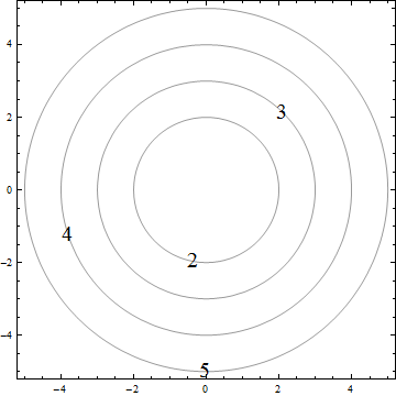
Using Cartesian parametrization and upper cone:
ContourPlot[x^2 + y^2, {x, -5, 5}, {y, -5, 5},
 ContourShading -> False, Contours -> {4, 9, 16, 25},
 ContourLabels -> (Text[Style[Sqrt[#3],20],{#1, #2}] &)]

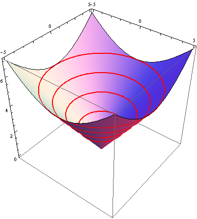
Using MeshFunctions:
Plot3D[Sqrt[x^2 + y^2], {x, -5, 5}, {y, -5, 5},
 MeshFunctions -> (#3 &), Mesh -> {Table[{j}, {j, 2, 5}]},
 BoxRatios -> {1, 1, 1}, MeshStyle -> {Thick, Red}]

Here is a link to approaches to combine both plots.
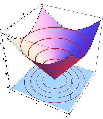
Combining (using approach from link):
cp = ContourPlot[x^2 + y^2, {x, -5, 5}, {y, -5, 5}, Frame -> False,
   Axes -> False, PlotRangePadding -> 0, Contours -> {4, 9, 16, 25},
   ContourShading -> False,
   ContourLabels -> (Text[Style[Sqrt[#3], 20], {#1, #2}] &),
   ContourStyle -> {{Thick, Red}}];
p1 = Plot3D[Sqrt[x^2 + y^2], {x, -5, 5}, {y, -5, 5},
   MeshFunctions -> (#3 &), Mesh -> {Table[{j}, {j, 2, 5}]},
   BoxRatios -> {1, 1, 1}, MeshStyle -> {Thick, Red}];


level = -1.2 10^-8; gr =
 Graphics3D[{Texture[cp], EdgeForm[],
   Polygon[{{-5, -5, level}, {5, -5, level}, {5, 5, level}, {-5, 5,
      level}},
    VertexTextureCoordinates -> {{0, 0}, {1, 0}, {1, 1}, {0, 1}}]},
  Lighting -> "Neutral"];
Show[p1, gr]

-
$\begingroup$ Isn't there a small coordinate mismatch between the ContourPlot and the 3D box? $\endgroup$ Commented Nov 13, 2013 at 10:18
-
2$\begingroup$ Yes, thank you...I did this in a rush to be illustrative and motivating, the texturing plot padding leads to the mismatch...you are absolutely right the non composed images should ok and I should have been more pedantic $\endgroup$– ubpdqnCommented Nov 13, 2013 at 10:22
-
$\begingroup$ Would you elaborate how
ContourLabels -> (Text[Style[Sqrt[#3],20],{#1, #2}] &)]works? $\endgroup$– user664Commented Oct 19, 2014 at 21:00
Analysis: Parameter u is the height z of a contour, so take the first two equations for a fixed value of u, e.g.:
ParametricPlot[{1.25 Cos[v], 1.25 Sin[v]}, {v, 0, 2 Pi}]
whose result, not shown here, is the expected circle.
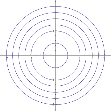
Implementation: For several heights, apply a function with the height as argument to a list of those heights, producing a list of individual circular images; then combine them all with Show:
 Show[(ParametricPlot[{# Cos[v], # Sin[v]}, {v, 0, 2 Pi},
 PlotRange -> {-2.25, 2.25}] &) /@ {0.5, 1, 1.25, 1.5, 1.75, 2}

Note that your syntax for the parametric equations had syntax errors: spaces missing between u and the trig function names; trig functions should be Cos and Sin, not cos and sin (built-in names begin with lower-case, and Mathematica is case-sensitive).
