How to work with differentials explicitly?

Question

When working with differential equations with independent (e.g. t )and dependent (e.g., x[t]) variables Mathematica expresses partial and 'regular' derivatives nicely, but not the derivative itself. Can anybody manage to do this?

I give an example: Let f depend on x, y and t. x and y depend on t. So, the partial derivative

with e.g. respect to x is in Matheamtica expressed by

f^(1,0,0)[x,y,t]

, the derivative with respect to the independent variable

as an example by

x'[t]

. But how can I make Mathematica to show the derivative e.g.

explicitly?

Answer 1

Dt is one way to work with differentials, unless you're after the more advanced functionality Timothy Wofford linked to in his comment. I'm not sure whether you want to do calculus with differentials, for instance in differential equations, or just want them to be formatted in a certain way.

Formatting

For formatting derivatives and differentials, these may be of help:

• How to make traditional output for derivatives
• Notation for implicit derivative

The derivative and Dt

The differential of a multivariable function:

w = f[x, y, t];
Dt[w]
(* Dt[t] * Derivative[0, 0, 1][f][x, y, t] + 
    Dt[y] * Derivative[0, 1, 0][f][x, y, t] + 
    Dt[x] * Derivative[1, 0, 0][f][x, y, t]   *)

The (matrix) derivative of f may be obtained with D

D[w, {{x, y, t}}]
(* {Derivative[1, 0, 0][f][x, y, t], 
    Derivative[0, 1, 0][f][x, y, t], 
    Derivative[0, 0, 1][f][x, y, t]}

The output of Dt[w] above may also be obtained with

D[w, {{x, y, t}}] . Dt[{x, y, t}]

One can substitute functions for x and y to make them explicitly depending on t, and the Chain Rule is automatically applied (of course):

Dt[w] /. {x -> x[t], y -> y[t]} // Factor // InputForm
(* Dt[t]*
    (Derivative[0, 0, 1][f][x[t], y[t], t] +
      y'[t]*Derivative[0, 1, 0][f][x[t], y[t], t] +
      x'[t]*Derivative[1, 0, 0][f][x[t], y[t], t])  *)

Differential equations and Dt

One can turn expressions in terms of Dt[x] etc. into differential equations:

dtToDE[diffForm_, vars_List, var_] /; MemberQ[vars, var] := 
  With[{indep = DeleteCases[vars, var]},
   0 == diffForm /. 
     Flatten[{Thread[Dt /@ indep -> D[Through[indep[var]], var]], 
       Thread[indep -> Through[indep[var]]]}] /. Dt[var] -> 1
   ];
dtToDE[diffForm_, vars_List, var_] := 
  D[Through[vars[var]], var] == 
   Extract[CoefficientList[diffForm, Dt /@ vars] /. 
     Thread[vars -> Through[vars[var]]], 
    1 + IdentityMatrix[Length[vars]]];

orthogonalTrajectory[diffForm_, vars_List] := 
  diffForm /. Thread[# -> Cross[#]] &[Dt /@ vars];

Examples

An exact differential.

Dt[x^2 + y^2 x - y^2]                            (* the differential of f *)
ode = dtToDE[Dt[x^2 + y^2 x - y^2], {x, y}, x]   (* as a derivative equation *)
DSolve[ode, y[x], x]                             (* solution to the ODE *)
Solve[x^2 + y^2 x - y^2 == C[1]/2, y]            (* solution to f = constant *)

(* 2 x Dt[x] + y^2 Dt[x] - 2 y Dt[y] + 2 x y Dt[y] *)
(* 0 == 2 x + y[x]^2 - 2 y[x] Derivative[1][y][x] + 2 x y[x] Derivative[1][y][x] *)
(* {{y[x] -> -(Sqrt[-2 x^2 - C[1]]/(Sqrt[2] Sqrt[-1 + x]))},
    {y[x] ->   Sqrt[-2 x^2 - C[1]]/(Sqrt[2] Sqrt[-1 + x])}}  *)
(* {{y    -> -(Sqrt[-2 x^2 + C[1]]/(Sqrt[2] Sqrt[-1 + x]))},
    {y    ->   Sqrt[-2 x^2 + C[1]]/(Sqrt[2] Sqrt[-1 + x])}}  *)

A differential with an integrating factor (pasted from an old test's TeX file, converted to a differential form with Dt):

ode = dtToDE[x dy + y dx + 4 x^3 y^4 dy /. {dx -> Dt[x], dy -> Dt[y]}, {x, y}, x]
sol = DSolve[ode, y[x], x];
ode /. {y'[x] -> Hold[D[y[x], x]]} /. sol // ReleaseHold // Simplify
Times @@ Subtract @@@ DeleteDuplicates@Simplify[x y^2 == x y[x]^2 /. sol] == 0 // Simplify

(* 0 == y[x] + x y'[x] + 4 x^3 y[x]^4 y'[x]   -- ODE *)
(* {True, True, True, True}                   -- all branches of sol satisfy the ODE *)
(* x^2 (4 y^4 - 2 y^2 C[1]) == 1              -- the integral curve (hacked from sol) *)

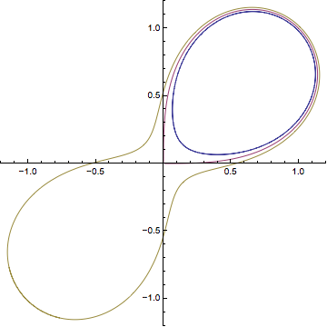
A system of equations, following three orthogonal trajectories to the gradient of a function.

sols = NDSolveValue[
         {dtToDE[orthogonalTrajectory[Dt[(x^2 + y^2)^2 - 4 x y], {x, y}], {x, y}, t],
          x[0] == #, y[0] == #},
         {x, y}, {t, -1.35, 1.35}] & /@ {0.99, 1., 1.01};
ParametricPlot @@ {Through[#[t]] & /@ sols, Flatten @ {t, sols[[1,1]]["Domain"]}}