1
$\begingroup$

How can I split in color classes, the pixels of an image that I load in Mathematica?

I would an output like this:

<Class1Name> 50% 
<Class2Name> 30% 
<Class3Name> 20%

The percentages refere to the amount of pixels of the image that are into that colour class.

The definition of the classes would be something like this: <Class1Name> = All pixels that are into a RGB range of colours (for example from a dark green to a light green)

I have tried a code like this:

Image[{List@@@DominantColors[<imagefile>, n]}, ImageSize -> 300]

But I don't know how to split the output in classes. By encreasing the value of $n$ I will have a better precision right? I would love also a plot of the normal distribution of the pixels, where in the $x$ axis lie the names of the classes and on the $y$ axis a normalized scale that go from 0 to 1. So the plot should look similar to this:
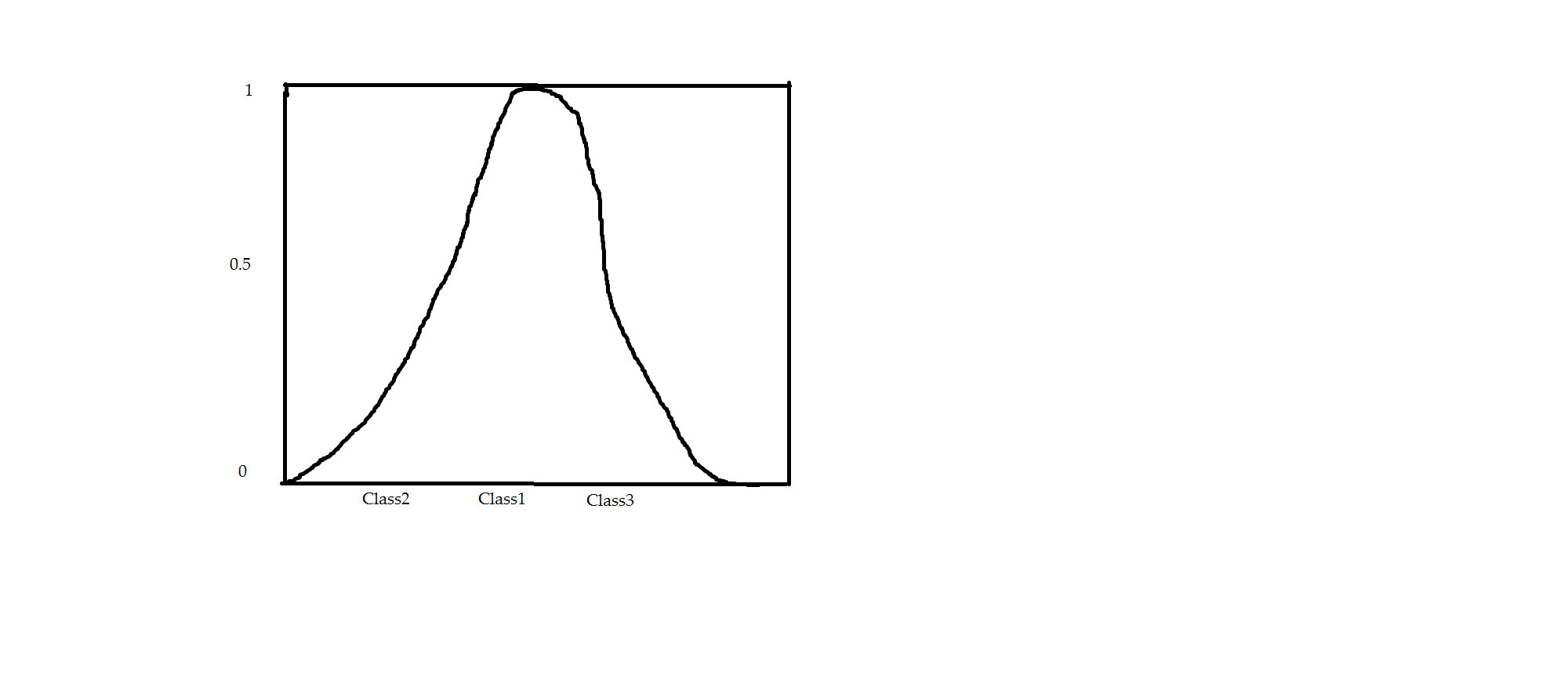
enter image description here

If is possible I would execute the computation of all this on the GPU or on both the CPU and GPU togheter, I would like to chose between an OpenCL and CUDA version of the code and if is not possible I would have a code optimized to perform the computation on all cores an threads of my CPU.

P.S. I have used in the examples only three classes but actually I would like to choose the number of classes that I prefer every time that I run the code.

$\endgroup$

2 Answers 2

7
$\begingroup$

One function you might find useful is PixelValuePositions. You can take an image img and find all the pixel positions where (say) Green occurs by

PixelValuePositions[img, Green, 0.1]

You could count how many there are by

Length[PixelValuePositions[img, Green, 0.1]]

and then calculate the percentages you wish. The third argument specifies how close to the given color a pixel must be in order to be counted. For example, the color

Green
RGBColor[0, 1, 0]

so the 0.1 means any pixel within 0.1 of {0,1,0}. You can see what these colors look like by choosing a bunch of them -- here you can plot 10 disks all within 0.1 color range of Green.

Table[Graphics[{RGBColor[#[[1]], 1 - #[[2]], #[[3]]] &@
    RandomVariate[UniformDistribution[{0, 0.1}], 3], Disk[]}], {i, 10}]
$\endgroup$
2
  • $\begingroup$ How can I have an idea of what range of Green for (example) will be counted if I choose (again, for example) $0.1$ as third argument? Can I have a preview of that green range? $\endgroup$
    – Aurelius
    Commented Aug 23, 2013 at 23:34
  • $\begingroup$ See the addition for a way to visualize the range of Greens within 0.1. $\endgroup$
    – bill s
    Commented Aug 24, 2013 at 0:10
6
$\begingroup$

I'm not sure if you plan to pre-define the colour classes or extract them from the image, but here is one way to do that latter.

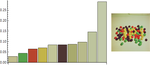
I use ColorQuantize to reduce the image to a palette of $n$ colours, then simply Tally the pixel values in the quantized image. The bar chart shows the fraction of pixels for each colour.

img = ExampleData[{"TestImage", "JellyBeans2"}];

n = 10;

q = ColorQuantize[img, n];
{colors, counts} = Transpose[Tally[ImageData[q] ~Flatten~ 1] ~SortBy~ Last];
BarChart[Normalize[counts, Total], ChartStyle -> RGBColor /@ colors] ~Legended~ img

enter image description here

$\endgroup$
1
  • $\begingroup$ You can see from your histogram that there are some classes---or column---that look similar to some others, for example the gray columns to the right. So, how can I put them into a single class that represent (say) all the Grays? $\endgroup$
    – Aurelius
    Commented Aug 24, 2013 at 9:48

Your Answer

By clicking “Post Your Answer”, you agree to our terms of service and acknowledge you have read our privacy policy.

Not the answer you're looking for? Browse other questions tagged or ask your own question.