4
$\begingroup$

I'm trying to reproduce the plots (Figure 1 and Figure 2) of this paper. The plots are obtained by solving the Eqs. 4.3 and 4.4. The boundary conditions described in section 3.3 for Eqn. 4.3 are provided as follows: $t'(u_0)= \infty$, $t'(u_k)=\pm \infty$ where $u_0$ is the turning point of the surface and $u_k$ denotes the deep IR. Similarly, the boundary conditions for Eqn. 4.4 are provided as, $t'(\infty)= 0$, $t'(u_k)=\pm \infty$. For all the plots, they have fixed $u_k=1$.

I'm using this code for Eqn. 4.3,

     uk = 1;
eom1 = t'[u] == 
   Sqrt[(u0^2 uk^3 - 
     u0^5)/((u^3 - uk^3) (u0^2 uk^3 - u0^5 - u^2 uk^3 + u^5))];
sol = ParametricNDSolve[{eom1, t'[u0] == 10^3, 
   t'[uk] == 10^3}, {t}, {u, 0, 2}, {u0}]
Plot[Evaluate[Im[t[u0][1] /. sol]], {u0, 0, 2}]

but it's not working.

Can anybody suggest how to proceed with the code?

$\endgroup$
4
  • 1
    $\begingroup$ This actually crashes the kernel. But if I remember, you can't have the parameter to ParametricNDSolve be the location of initial conditions. I think this came up before. I remember such question. Why are you using the parameter as the location of initial condition? Also this is first order ode and you are giving 2 constrains. This will give an error. The IC should also not be first order derivative, since the ode itself is first order. $\endgroup$
    – Nasser
    Commented May 6 at 6:38
  • $\begingroup$ Those are boundary conditions; I don't know about the IC. $\endgroup$ Commented May 6 at 11:53
  • $\begingroup$ (1) You have two BCs for a first-order ODE. It seems over determined to me. (2) An IC is just a BC at which the numerical integration starts. You can control this by looking up the options for the "Shooting" method in the docs; otherwise, NDSolve picks one of the BCs for part of the ICs and fills in values as needed in higher-order systems. $\endgroup$
    – Goofy
    Commented May 6 at 12:20
  • $\begingroup$ The crash is reported as a bug. $\endgroup$ Commented May 7 at 15:53

1 Answer 1

5
$\begingroup$

We can use NIntegrate instead of NDSolve as follows

uk = 1;(*b=u0^2 uk^3-u0^5*);
t[u1_?NumericQ, u2_?NumericQ, b_?NumericQ, t0_, pm_] := 
 pm  NIntegrate[
    Sqrt[(b)/((u^3 - uk^3)  (b - u^2  uk^3 + u^5))], {u, u2, uk, u1}, 
    Method -> "LocalAdaptive", Exclusions -> {u - uk == 0}] + t0

Then we can play with parameters and Re,Im to plot parts of trajectory, for example

plot1 = Quiet@
  ParametricPlot[{{u1, Re[t[u1, -2, 1, 0, 1]]}, {u1, 
     Re[t[u1, -2, 1, 0, -1]]}}, {u1, 1, 2}, PlotStyle -> {Blue, Blue},
    PlotRange -> {{0, 2}, {-2, 2}}, AspectRatio -> 1/2];

plot2 = Quiet@
  ParametricPlot[{{u1 - .19, Im[t[u1, 1, -1, -.5  I, 1]]}, {u1 - .19, 
     Im[t[u1, 1, -1, .5  I, -1]]}}, {u1, 1.19, 2.2}, 
   PlotStyle -> {Green, Green}, PlotRange -> {{0, 2}, {-2, 2}}];

Show[ParametricPlot[{uk, u}, {u, -2, 2}, PlotStyle -> {Black, Thin}, 
  PlotRange -> {{.8, 2}, {-2, 2}}, AspectRatio -> 1/2], plot1, plot2] 
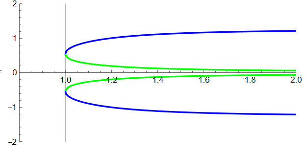
Figure 1

Update 1. To compute red lines we use

uk = 1;
t[u1_?NumericQ, u2_?NumericQ, b_?NumericQ, t0_, pm_] := 
  pm NIntegrate[
     Sqrt[(b)/((u^3 - uk^3) (b - u^2 uk^3 + u^5))], {u, u2, uk, u1}, 
     Method -> "LocalAdaptive", Exclusions -> {u - uk == 0}] + t0;

plot = Table[
  Quiet@ParametricPlot[
    Table[{u1, 
      Re[t[u1, x, x^2 uk^3 - x^5, 0, m]]}, {m, {-1, 1}}], {u1, 1, x}, 
    PlotStyle -> Red, PlotRange -> {{0.5, 5}, {-2, 2}}, 
    AspectRatio -> 1/2], {x, 1.5, 4, .5}]
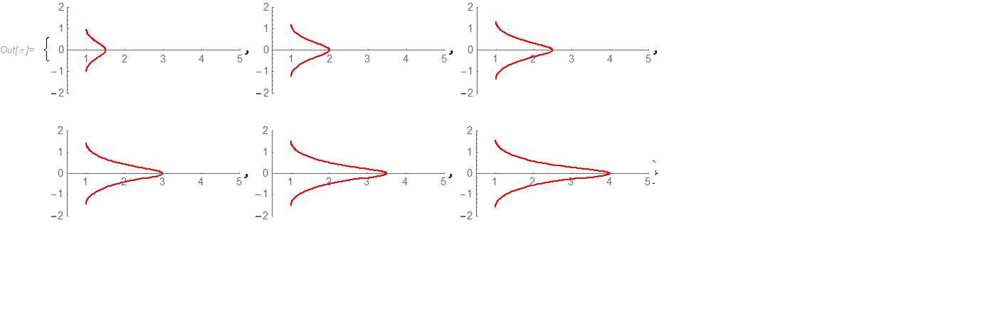
Figure2

Also we can use NDSolve as follows

sol[u0_] := 
 Module[{uk = 1, e = 10^-5}, 
  s = NDSolve[{t'[
        u]^2 == (u0^2 uk^3 - 
         u0^5)/((u^3 - uk^3) (u0^2 uk^3 - u0^5 - u^2 uk^3 + u^5)), 
     t[u0 - e] == 0}, t, {u, uk + e, u0 - e}]; s]

Table[Quiet@
  ParametricPlot[
   Table[{u1, Re@Evaluate[t[u1] /. sol[x][[m]][[1]]]}, {m, 2}], {u1, 
    1, x}, PlotStyle -> Red, PlotRange -> {{0.5, 5}, {-2, 2}}, 
   AspectRatio -> 1/2], {x, 1.5, 4, .5}]
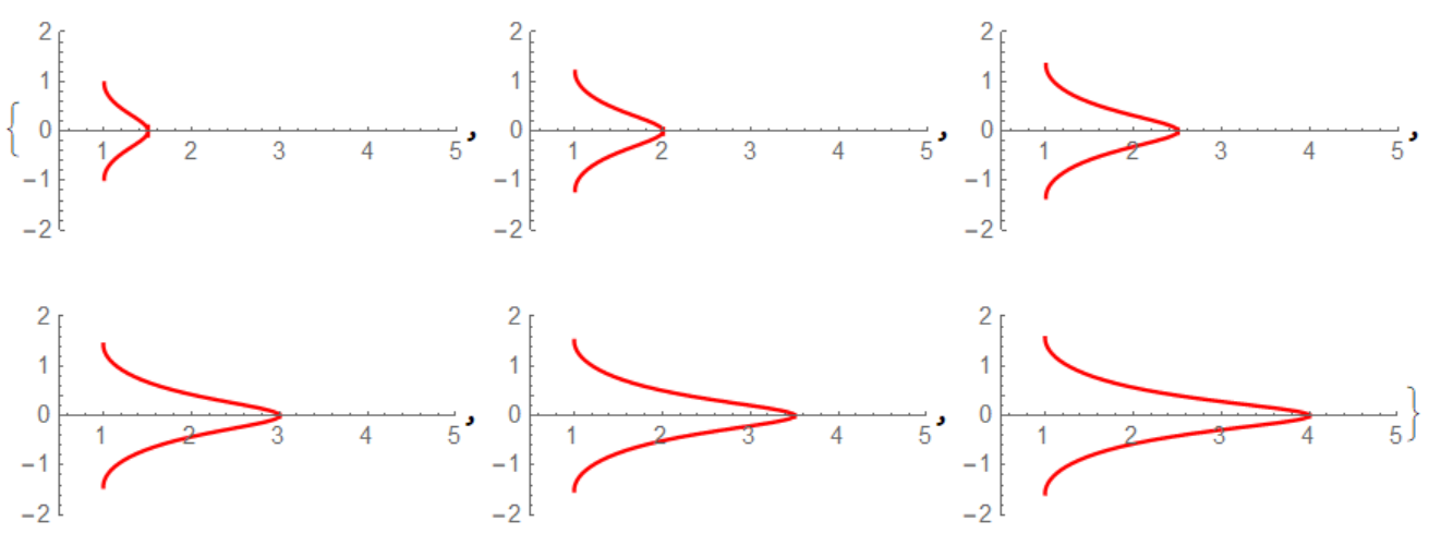
Figure 3

$\endgroup$
5
  • $\begingroup$ Thank you very much for your answer. Could you suggest how to get the red colour plot as shown in the image on page no. 13 of the linked paper? $\endgroup$ Commented May 6 at 13:23
  • $\begingroup$ Is there no use for $u_0$ here, or are you taking $u_0$ as $u_2$? As we'll proceed further in the linked paper, they have done plots for different values of $u_0$ as shown in the image; how should we proceed in that case? $\endgroup$ Commented May 6 at 14:22
  • $\begingroup$ I've some queries, like what is $t_0$, is it required to cancel the divergence, and how did you select specific values of $t_0$, like in plot1 you chose the value as 0 and in plot2 as $±0.5i$ $\endgroup$ Commented May 7 at 5:13
  • $\begingroup$ @EntangledQuark Please see Update 1 to my answer. $\endgroup$ Commented May 7 at 12:06
  • $\begingroup$ I appreciate your response significantly. $\endgroup$ Commented May 7 at 13:51

Your Answer

By clicking “Post Your Answer”, you agree to our terms of service and acknowledge you have read our privacy policy.

Not the answer you're looking for? Browse other questions tagged or ask your own question.