7
$\begingroup$

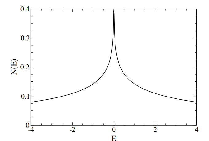
I am trying to plot the density of states $$ N(E)= \frac{1}{N}\Sigma_{k} (\delta{(E - \epsilon_{k}))} $$ where $\epsilon_{k} = -2t*[cos(k_x)+cos(k_y)]$ and $k$ goes from $-\pi$ to $\pi$. For this plot, we will get a singular point when E = 0 and it will peak at this point. This is done for a 2D Hubbard Model without considering the disorder. This is the plot I am expected to get -

enter image description here

My code:

energy[kx_, ky_] := -2  t  (Cos[kx] + Cos[ky]);

nPoints = 100;
kRange = Range[-Pi, Pi, 2  Pi/(nPoints - 1)];

energyValues = 
  Flatten[Table[energy[kx, ky], {kx, kRange}, {ky, kRange}]];

densityOfStates[
   Ee_] := (1/Length[energyValues])  Sum[
    DiracDelta[Ee - en], {en, energyValues}];

Plot[densityOfStates[Ee], {Ee, -4, 4}, PlotRange -> All, 
 AxesLabel -> {"E", "N(E)"}, PlotRange -> {{-4, 4}, {0, 0.5}}]

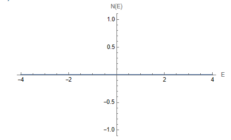
This is the plot I am getting -

enter image description here

I am implementing this paper - https://www.cond-mat.de/events/correl16/manuscripts/scalettar.pdf

$\endgroup$
7
  • $\begingroup$ DiracDelta is the implementation of the $\delta$-distribution in Mathematica, not a usual function. Its plots make no sense. $\endgroup$
    – user64494
    Commented Apr 27 at 12:59
  • $\begingroup$ @user64494 Oh okay, could you please suggest any other way I can implement this? Thanks $\endgroup$ Commented Apr 27 at 13:15
  • $\begingroup$ What is t? How can you plot anything when you miss the definition of t? $\endgroup$ Commented Apr 27 at 13:52
  • 1
    $\begingroup$ I am voting to reopen this question because unlike the linked post, it is not demanded here to get the density of states using a numerical integration and differentiation. Moreover, there are powerful mathematical methods to address exactly this kind of problems, see for instance, Rev. Mod. Phys. 78, 275 (2006), doi: 10.1103/RevModPhys.78.275. $\endgroup$
    – yarchik
    Commented Sep 5 at 8:28
  • 1
    $\begingroup$ I will provide an implementation of the kernel polynomial method for the density of states if the question is reopened. $\endgroup$
    – yarchik
    Commented Sep 5 at 8:31

4 Answers 4

6
$\begingroup$

As has been noticed in other answers, the brute force method is quite slow. One way to deal with the evaluation of a large sum of delta functions is to expand the density of states in terms of orthogonal polynomials. Since the range of energies is finite, the Chebyshev polynomials $T_n(x)$ is an obvious choice. Quite generally, a function $f:[-1,1]\rightarrow \mathbb{R}$ can be written as a sum $$ f(x)=\frac{1}{\pi\sqrt{1-x^2}}\left[\mu_0+2\sum_n\mu_nT_n(x)\right], $$ where $\mu_n$ are the moments computed according to: $$ \mu_n=\int_{-1}^1f(x)T_n(x)dx. $$ It is clear that in the case of $f$ given by a sum of delta functions, the integral is trivial. In principle, this already gives a prescription. However, when the polynomial sum is truncated, the resulting density of states suffers from fluctuations—also known as Gibbs oscillations. One way to deal with this problem is to suppress the weight of higher order polynomials with the $g_n$ factors: $$ f(x)=\frac{1}{\pi\sqrt{1-x^2}}\left[\mu_0g_0+2\sum_n^N\mu_ng_nT_n(x)\right]. $$ In Rev. Mod. Phys. 78, 275 (2006), it is shown what that the optimal form of the factors is: $$ g_n=\frac{(N+2-n) \cos \left(\frac{\pi n}{N+2}\right)+\cot \left(\frac{\pi }{N+2}\right) \sin \left(\frac{\pi n}{N+2}\right)}{N+2}. $$ This leads to the following code:

DOScb[evals_,Ncb_,Nint_]:=Module[{eSorted,neng,xvals,emn, emx,μcb,gcb,itab,de},
  eSorted=Sort[evals];
  emn=eSorted[[1]]-0.5;
  emx=eSorted[[-1]]+0.5;
  neng=Length[eSorted];
  xvals=2(eSorted-emn)/(emx-emn)-1;
  de=2./(Nint-1);
  μcb=Table[Total[ChebyshevT[n,#]&/@xvals]/neng,{n,Ncb}];
  gcb=Table[N[1/(Ncb+2)*((Ncb+2-n)*Cos[π*n/(Ncb+2)]+Sin[π*n/(Ncb+2)]Cot[π/(Ncb+2)])],{n,Ncb}];
  itab=Table[{emn+(x+1.)*(emx-emn)/2,2/(emx-emn)*1/(π*Sqrt[1-x^2])*(1+2*Sum[μcb[[n]]*gcb[[n]]*ChebyshevT[n,x],{n,Ncb}])},{x,-1.+de,1.-de,de}];
  Interpolation[itab,"ExtrapolationHandler"->{0&,"WarningMessage"->False}]
  ]

The function takes 3 arguments: a set of energies, the highest order of included Chebyshev polynomial, and the number of points for interpolation of the final result.

By chance, the exact analytic solution is also known:

$$ n(E)=\frac{1}{2 \pi ^2}K(1-(E/4)^2) \theta (4-|E| ), $$ where $\theta$ is the Heaviside function and $K$ is an elliptic integral.

Below, I compare density of states computed using 250 Chebyshev polynomials with the analytic expression

t = 1.;
energy[kx_, ky_] := -2 t (Cos[kx] + Cos[ky]);
nkp = 150;
dk = 2*Pi/(nkp - 1);
energyValues = 
  Flatten[Table[
    energy[kx, ky], {kx, -Pi, Pi, dk}, {ky, -Pi, Pi, dk}]];
dos2d = DOScb[energyValues, 250, 1001]

dosExact[w_] := HeavisideTheta[4 - Abs[w]]/(2*Pi^2)*EllipticK[1 - (w/4)^2]

Plot[{dosExact[w], dos2d[w]}, {w, -4.5, 4.5}, 
 PlotTheme -> {"Frame", "Monochrome"}, 
 PlotRange -> All, 
 Exclusions -> None, 
 PlotStyle -> {Automatic, Red}]
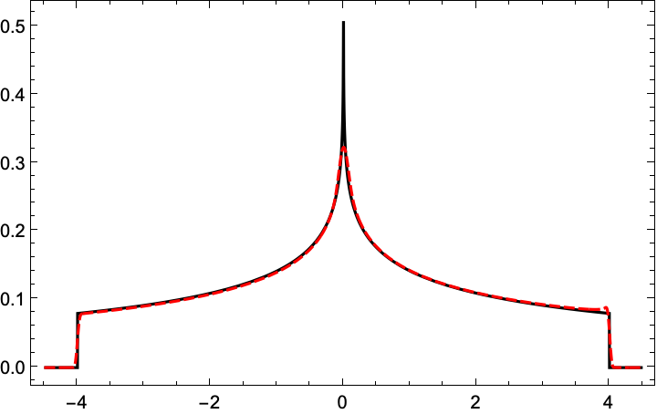
density of states

$\endgroup$
1
  • 1
    $\begingroup$ Brilliant answer! $\endgroup$
    – ubpdqn
    Commented Sep 11 at 22:37
5
$\begingroup$

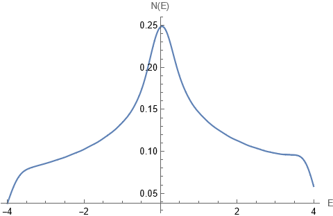
I used function dirac as approximation to Dirac delta. Dirac delta is limit as a->0. I used value a->1/3 and nPoints = 30. For larger number of points the code is slow and for smaller value of a there are overflows errors.

The plot is quite similar but still not same as in OP. So I guess there might be some mistakes in OP code or they used in the paper a different approximation for Dirac delta.

t = 1.;
dirac[x_] := 1/(a Sqrt[Pi]) E^-(x/a)^2 /. a -> 1/3

energy[kx_, ky_] := -2 t (Cos[kx] + Cos[ky]);

nPoints = 30;
kRange = Range[-Pi, Pi, 2 Pi/(nPoints - 1)];

energyValues = 
  Flatten[Table[energy[kx, ky], {kx, kRange}, {ky, kRange}]];

densityOfStates[
   Ee_] := (1/Length[energyValues]) Sum[
    dirac[Ee - en], {en, energyValues}];

Plot[densityOfStates[Ee], {Ee, -4, 4}, PlotRange -> All, 
 AxesLabel -> {"E", "N(E)"}, PlotRange -> {{-4, 4}, {0, 0.5}}]

enter image description here

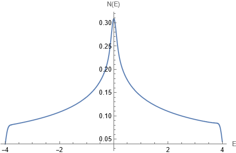
With a->1/10 in dirac[x_] := 1/(a Sqrt[Pi]) E^-(x/a)^2 /. a -> 1/10 and nPoints = 200 the plot resembles the OP image quite well. For smaller a and larger nPoints I am sure it can be even better but the code is slow.

enter image description here

$\endgroup$
5
  • $\begingroup$ This is wishful thinking. Replacing a->1/3 by a->1/10, one obtains something strange. For the user's convenience I add the result to your answer. $\endgroup$
    – user64494
    Commented Apr 27 at 17:47
  • 6
    $\begingroup$ Can moderators block this user to stop modifying my answer with useless edits? $\endgroup$ Commented Apr 27 at 17:51
  • $\begingroup$ See the screen with my addition to the azerbajdzan's answer. $\endgroup$
    – user64494
    Commented Apr 27 at 17:58
  • $\begingroup$ To those who can not read with comprehension. The code depends also on number of nPoints not only on approximation factor a of Dirac delta. When a is decreased the number of points nPoints must be increased appropriately. $\endgroup$ Commented Apr 27 at 18:11
  • $\begingroup$ Indeed, with a->1/10 and nPoints=100; the result is better than yours. I repeat that a good code is a commented code. $\endgroup$
    – user64494
    Commented Apr 27 at 18:21
5
$\begingroup$

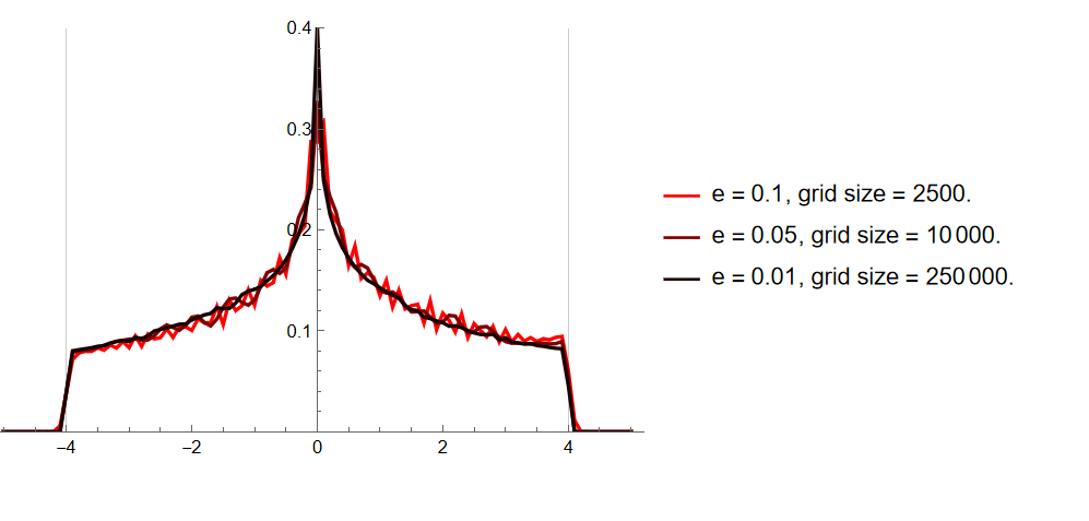
This is an extended comment to support the answer by @azerbajdzan (and his comments). I have voted for @azerbajdzan answer. Using the dirac delta distribution approximation. As @azerbajdzan comments it depends on choices. It is a different implementation (probably slower) but the motivation is illustrative. The point is better approximations of the density of states for finer meshes require better delta distribution approximations.

d[x_, e_] := Exp[-(x/e)^2]/(e   Sqrt[Pi])
mesh[n_] := -2 (Cos[#1] + Cos[#2]) & @@@ 
  Tuples[Subdivide[-Pi, Pi, n - 1], 2]
func[en_, e_, n_] := Chop[Total[d[en - #, e] & /@ mesh[n]]/n^2]
gr = Show[
   Quiet@Table[
     ListPlot[Table[{j, Evaluate@func[j, k, 5/k]}, {j, -5, 5, 0.1}], 
      Joined -> True, GridLines -> {{-4, 4}, None}, 
      PlotRange -> {0, 0.4}, 
      PlotStyle -> RGBColor[10 k, 0, 0]], {k, {0.1, 0.05, 0.01}}]];


Legended[gr,
 LineLegend @@ 
  Transpose[
   Table[{RGBColor[10 k, 0, 0], 
     Row[{"e = ", k, ", grid size = ", 25/k^2}]}, {k, {0.1, 0.05, 
      0.01}}]]]

enter image description here

$\endgroup$
2
$\begingroup$

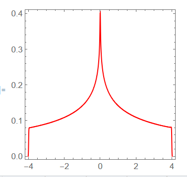
Well, in such case to avoid the summation process, we can use the magical SmoothHistogram which takes 2 sec as follows:

energy[kx_, ky_] := -2  (Cos[kx] + Cos[ky]);
nPoints = 1000.;
kRange = Range[-Pi, Pi, 2 Pi/(nPoints - 1)];
energyValues = 
  Flatten[Table[energy[kx, ky], {kx, kRange}, {ky, kRange}]];
SmoothHistogram[energyValues, 0.01, Frame -> True, Axes -> False, 
 PlotStyle -> Directive[Red, AbsoluteThickness[1.2]], 
 ImageSize -> 200, AspectRatio -> 1]       

enter image description here

$\endgroup$

Your Answer

By clicking “Post Your Answer”, you agree to our terms of service and acknowledge you have read our privacy policy.

Not the answer you're looking for? Browse other questions tagged or ask your own question.