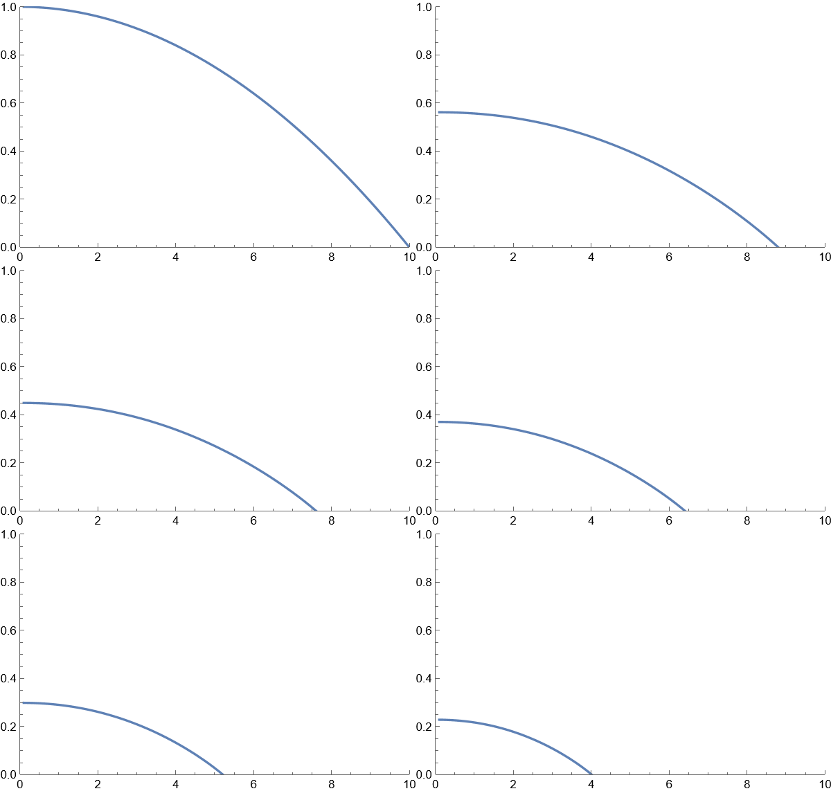
Recently I've come across the following system governing the spreading of an evaporating droplet. The height of the droplet $h$ is defined by the following equation
$$\frac{\partial h}{\partial t}=-\frac{1}{r}\frac{\partial }{\partial r}\left(- \frac{r h^3}{3\mu}\frac{\partial p}{\partial r}\right)-j(r,t)$$
Which is a clear, solvable 1D Partial-Differential Equation solvable by the Method of Lines.
The evaporation rate, $j(r,t)$, however is given as a solution to the following 2D Laplace Equation:
$$\nabla^2 c(r,z,t)=0$$ $$j(r,t)=\alpha \frac{\partial c(r,0,t)}{\partial z}$$
With boundary conditions $$c(r,0,t)=h(r,t) \ for \ r < R(t)$$ $$\frac{\partial c(r,0,t)}{\partial z}=0 \ for \ r> R(t)$$ $$c(r,z,t)=0 \ for \ r\rightarrow \infty, z \rightarrow \infty$$
While I'm able to solve the spreading of the droplet, as well as the evaporation due to an abitrary concentration field independently, I have no idea how to couple the two solutions together. The two way coupling is particularly annoying as
- The solutions of the height field is used as the boundary condition of the Laplace equation;
- The solution of the Laplace equation gives the evaporation rate which affects the height field.
I'll appreciate any advice to go forward on this problem. Below are my current code are both the spreading of the Droplet and the Evaporation of an arbitrary concentration field. Thanks!
Droplet Spreading Code
Note that the pdetoode package by xzczd is used. For sake of clarity of code that part is not included.
(*Definitions*)

(*Constants*)
\[Mu] = 2.75*10^-6 (*mN mm^-2 s*);(*Viscosity of water*)
\[Gamma] = 0.072(*mN mm^-1*);(*Air-water surface tension*)
\[Beta] = 1(*mm s^-1*);(*Slip constant*)

(*Grid specification*)
difforder = 2;
lb = 1/100; rb = 1; points = 100;
grid = Array[# &, points, {lb, rb}];

unitStepExpand = Simplify`PWToUnitStep@PiecewiseExpand@# &;

With[{h = h[r/R[t] , t], q = q[r/R[t], t], p = p[r/R[t], t], R = R[t]},

 (*Equations neglecting evaporation*)
 EqnP = Simplify[
    p == \[Gamma] (-D[h, r, r] -
        unitStepExpand@If[x < 1/20, D[h, r, r], D[h, r]/r])] /.
   r -> x R;
 EqnQ = Simplify[q == (r h^3)/(3 \[Mu]) (-D[p, r])] /. r -> x R;
 EqnC = Simplify[ D[h, t] == -(1/r) D[ q, r]] /. r -> x R;
 EqnR = D[R, t] == \[Beta] (-D[h, r]^3 - 1) /. r -> R;]

(*Boundary conditions*)
dr = R[t] lb;

EqnBC1 = {D[r h[lb, t] dr, t] + r q[lb, t] == 0} /. r -> lb R[t];
EqnBC2 = {Derivative[1, 0][h][lb, t] == 0};
EqnBC3 = {h[rb, t] == 0};

(*Initial conditions*)
EqnIC = {h[x, 0] == (1 - x^2)};

(*Equation Discretisation*)
removeredundant = #[[3 ;; -2]] &;

tfunc = pdetoode[{p, q, h}[x, t], t, grid, difforder];
odemid = Map[tfunc, {EqnP, EqnQ}, {2}];
odeC = Block[{p, q}, Set @@@ odemid; tfunc@EqnC] // removeredundant;

odeBC1 = Block[{p, q}, Set @@@ odemid; tfunc@EqnBC1];
odeBC2 = With[{sf = 100}, diffbc[t, sf]@EqnBC2 // tfunc];
odeBC3 = With[{sf = 100}, diffbc[t, sf]@EqnBC3 // tfunc];

odeR = Block[{p, q}, Set @@@ odemid; tfunc@EqnR];

odeIC = Append[EqnIC // tfunc, R[0] == 10];

(*Solving the equations*)
var = {h /@ grid, R};

Monitor[sollst =
   NDSolveValue[{odeC, odeR, odeBC1, odeBC2, odeBC3, odeIC},
    var, {t, 0, 6}, EvaluationMonitor :> (time = t),
    Method -> {"EquationSimplification" -> "Solve"},
    WorkingPrecision -> 20, MaxSteps -> Infinity], time];

{hsol} = rebuild[#, grid, 2] & /@ {sollst[[1]]}
Rsol = sollst[[2]]

(*Visualising Solutions*)
Manipulate[
 Plot[hsol[Abs[r]/Rsol[t], t], {r, 1/10, Rsol[t]},
  PlotRange -> {{0, 10}, {0, 3}}], {t, 0, 1}]
Evaporation Code
Needs["NDSolve`FEM`"]

(*Mesh Generation*)
L = 10;
H = 5;

l1 = ToGradedMesh[
  Line[{{0}, {L}}], <|"Alignment" -> "Left", "ElementCount" -> 40|>]
h1 = ToGradedMesh[
  Line[{{0}, {H}}], <|"Alignment" -> "Left", "ElementCount" -> 20|>]

mesh = ElementMeshRegionProduct[l1, h1]

(*Arbitrary height function*)
h[x_] := 1 - x^2;

(*Solving Equations*)
EqnC = 1/x D[x Derivative[1, 0][c][x, y], x] +
    Derivative[0, 2][c][x, y] ==
   NeumannValue[0, y == 0 && Abs[x] > 1] + NeumannValue[0, y == H] +
    NeumannValue[0, Abs[x] == L];
EqnB = DirichletCondition[c[x, y] == h[x], Abs[x] <= 1 && y == 0];
EqnB2 = DirichletCondition[c[x, y] == 0, y == H];
EqnB3 = DirichletCondition[c[x, y] == 0, Abs[x] == L];

csol = NDSolveValue[{EqnC, EqnB, EqnB2, EqnB3},
  c, {x, y} \[Element] mesh]
j[r_] := \[Alpha] (csol[r, 0] - csol[r, 0.001])/0.001

(*Visualising Results*)
Plot[j[x] /. \[Alpha] -> 1, {x, 0, 10}, PlotRange -> All]


