8
$\begingroup$

I am trying to construct basins of attraction using the newton's method for the system of two equations whose roots are real. I need to develop a code to get basin of attraction. Unfortunately, my code does not work. Can anyone please help me find the error in my code? I don't understand what exactly the problem is. My code for the basins of attraction is given below:

ClearAll["Global`*"]
r1 = {-1, -1};
r2 = {0, 0};
r3 = {1, 1};

x = Range[-2, 2, 0.02];
y = Range[-2, 2, 0.02];

Xr1 = {}; Xr2 = {}; Xr3 = {}; Xr4 = {};

Do[Do[X0 = {x[[i]], y[[j]]};
X = {x[[i]], y[[j]]};
NoIter = 5;
Do[f = {X[[1]]^3 - X[[2]], X[[2]]^3 - X[[1]]};
 Jf = {{3*X[[1]]^2, -1}, {-1, 3*X[[2]]^2}};
 X = X - Inverse[Jf].f, {NoIter}];
If[Norm[X - r1] < 1 e - 25, Xr1 = Append[Xr1, X0], 
 If[Norm[X - r2] < 1 e - 25, Xr2 = Append[Xr2, X0], 
  If[Norm[X - r3] < 1 e - 25, Xr3 = Append[Xr3, X0], 
   Xr4 = Append[Xr4, X0]]]], {j, Length[y]}], {i, Length[x]}];

ListPlot[{Xr1, Xr2, Xr3, Xr4}, PlotStyle -> {Red, Blue, Green, Black},
AspectRatio -> 1, PlotRange -> {{-2, 2}, {-2, 2}}, Frame -> True, 
FrameLabel -> {"x", "y"}, PlotLegends -> {"r1", "r2", "r3", "r4"}, 
PlotLabel -> 
"Basin of attraction for f(x,y) = x^3-y = 0 and y^3-x=0"] 


$\endgroup$
10
  • 1
    $\begingroup$ Change 1 e -25to 10^-25! $\endgroup$ Commented Mar 15 at 7:44
  • $\begingroup$ And you don't calculate the Jacobian correctly. Just try Clear[x, y]; D[{x^3 - y , y^3 - x}, {{x, y}}] and compare the result to yours. $\endgroup$
    – xzczd
    Commented Mar 15 at 7:51
  • $\begingroup$ I have made these changes, but it doesn't work. $\endgroup$
    – onk
    Commented Mar 15 at 8:38
  • $\begingroup$ That should not happen. How did you change your code? $\endgroup$
    – xzczd
    Commented Mar 15 at 8:42
  • $\begingroup$ I changed as below: Jf = D[{X[[1]]^3 - X[[2]], X[[2]]^3 - X[[1]]}, {{X[[1]], X[[2]]}}]; X = X - Inverse[Jf].f, {NoIter}]; $\endgroup$
    – onk
    Commented Mar 15 at 9:04

3 Answers 3

8
$\begingroup$

The simplest way is to use FindRoot with option Method -> {"Newton", "StepControl" -> Automatic} and with random initial points as follows

varALL = {x, y}; eqAll = {x^3 - y, y^3 - x};
points := 
 Module[{res, evx}, {res, {evx}} = 
   Reap[FindRoot[Table[eqAll[[i]] == 0, {i, Length[eqAll]}], 
     Table[{varALL[[i]], RandomReal[{-2, 2}]}, {i, Length[varALL]}], 
     Method -> {"Newton", "StepControl" -> Automatic}, 
     MaxIterations -> 1000, EvaluationMonitor :> Sow[varALL]]]; evx]

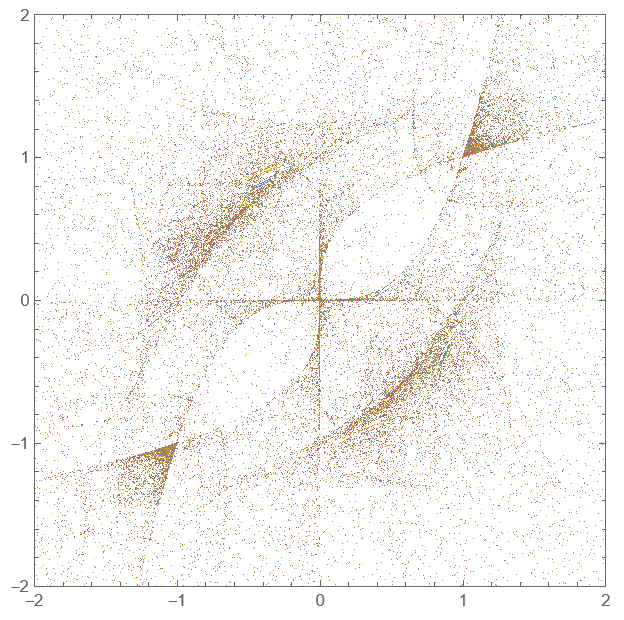
With this code we can generate list of points in Newton's iterations and plot basins of attraction

lst = Table[points, {5000}];
ListPlot[Evaluate[lst], Frame -> True, 
 PlotRange -> {{-2, 2}, {-2, 2}}, AspectRatio -> 1, Axes -> False]

Figure 1

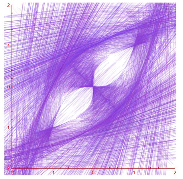
We also can use Line for visualization as follows

varALL = {x, y}; eqAll = {x^3 - y, y^3 - x};
line := Module[{res, evx}, {res, {evx}} = 
   Reap[FindRoot[Table[eqAll[[i]] == 0, {i, Length[eqAll]}], 
     Table[{varALL[[i]], RandomReal[{-2, 2}]}, {i, Length[varALL]}], 
     Method -> {"Newton", "StepControl" -> Automatic}, 
     MaxIterations -> 1000, EvaluationMonitor :> Sow[varALL]]]; 
  Line[evx]]

Graphics[
 Evaluate[
  Table[{RGBColor[RandomReal[{0.4, .7}], RandomReal[{.1, .4}], 
     RandomReal[{.7, 1}], .1], line}, {2000}]], Frame -> False, 
 Axes -> True, PlotRange -> {{-2, 2}, {-2, 2}}, 
 AxesOrigin -> {-2, -2}, AxesStyle -> Red]

Figure 2

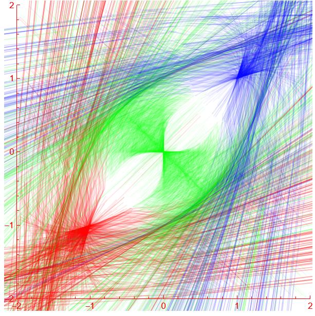
To colorize last picture with RGBColor we use code

lst = Table[point, {2000}];

root0 = Select[lst, Norm[Last[#]] < 10^-6 &];

root1 = Select[lst, Abs[Last[#][[1]] - 1] < 10^-6 &];

rootm1 = Select[lst, Abs[Last[#][[1]] + 1] < 10^-6 &];
Graphics[{{RGBColor[1, 0, 0, .1], 
   Line[rootm1]}, {RGBColor[0, 1, 0, .05], 
   Line[root0]}, {RGBColor[0, 0, 1, .05], Line[root1]}}, 
 Frame -> False, Axes -> True, PlotRange -> {{-2, 2}, {-2, 2}}, 
 AxesOrigin -> {-2, -2}, AxesStyle -> Red]

Figure 2

$\endgroup$
8
$\begingroup$

modified

Try

xygrid = Flatten[
   Outer[{#1, #2} &, Subdivide[-2, 2, 250 ], Subdivide[-2, 2, 250]], 
   1];
lsg = Table[ {xyi, {x, y} /. 
     FindRoot[{x^3 - y == 0, -x + y^3 == 0}, {{ x, xyi[[1]]}, { y, 
        xyi[[2]]}} , 
      Method -> {"Newton"(*,"StepControl"\[Rule]Automatic*)}, 
      MaxIterations -> 100  ]} , {xyi,  xygrid   }]  ;

fp = {{0, 0}, {1, 1}, {-1, -1}};
fp1 = Select[lsg, (#[[2]] - fp[[1]]) . (#[[2]] - fp[[1]]) < .001 &];
fp2 = Select[lsg, (#[[2]] - fp[[2]]) . (#[[2]] - fp[[2]]) < .001 &];
fp3 = Select[lsg, (#[[2]] - fp[[3]]) . (#[[2]] - fp[[3]]) < .001 &];

Graphics[{PointSize[Small], Red , Point[fp1[[All, 1]]], Green , 
Point[fp2[[All, 1]]], Blue , Point[fp3[[All, 1]]], FaceForm[Red], 
EdgeForm[Black], Disk[fp[[1]], .05], FaceForm[Green], 
Disk[fp[[2]], .05], FaceForm[Blue], Disk[fp[[3]], .05]}]

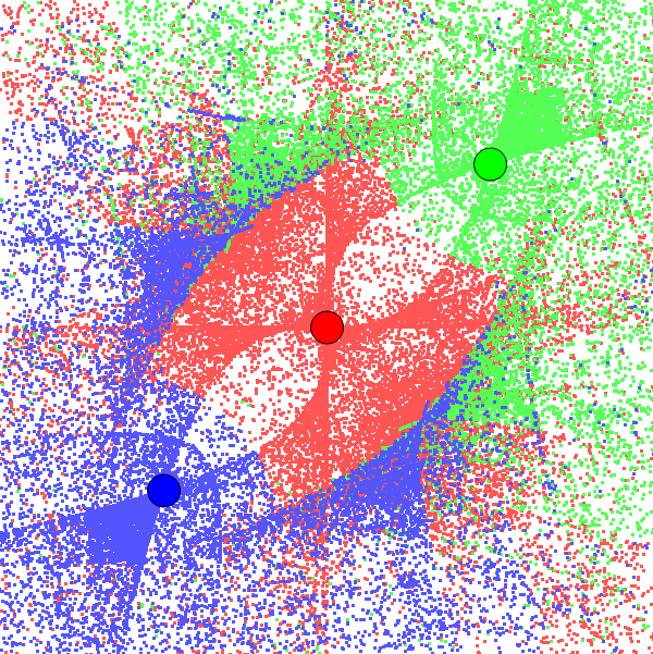
enter image description here

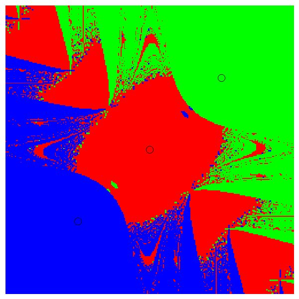
addendum

Colorize @AlexTrounev`s fine solution approach

lsg = Table[{ fp, {pts}} = 
    Reap[FindRoot[{x^3 - y == 0, -x + y^3 == 0}, {{ x, 
        RandomReal[{-2, 2}]}, { y, RandomReal[{-2, 2}]}} , 
      Method -> {"Newton"(*,"StepControl"\[Rule]Automatic*)}, 
      MaxIterations -> 1000, 
      EvaluationMonitor :> Sow[varALL]]] , {10000}];
fixp = {{0, 0}, {1, 1}, {-1, -1}};
erg = Map[{Values[#[[1]]], Flatten[#[[2]], 1]} &, lsg] // Chop;
fp1 = Select[erg, #[[1]] == fixp[[1]] &][[All, 2]]  // Flatten[#, 1] &;
fp2 = Select[erg, #[[1]] == fixp[[2]] &][[All, 2]]  // Flatten[#, 1] &;
fp3 = Select[erg, #[[1]] == fixp[[3]] &][[All, 2]]  // Flatten[#, 1] &;
Graphics[{PointSize[Small], Lighter[Red], Point[fp1 ], Lighter[Green],
   Point[fp2 ], Lighter[Blue], Point[fp3 ], PointSize[Large], 
  FaceForm[Red], EdgeForm[Black], Disk[fixp[[1]], .1], 
  FaceForm[Green], Disk[fixp[[2]], .1], FaceForm[Blue], 
  Disk[fixp[[3]], .1]}, PlotRange -> {{-2, 2}, {-2, 2}}]

enter image description here

addendum 2

The last plot depends on the plotting order of fp1,fp2,fp3, because pixel may overlap because of numerical reasons!

list = {{ Red , Point[fp1 ]}, { Green , Point[fp2 ]}, { Blue , 
    Point[fp3 ]}};
GraphicsRow[
 Map[Graphics[{PointSize[.001],Permute[list, #]  , FaceForm[Red], EdgeForm[Black], 
     Disk[fixp[[1]], .1], FaceForm[Green], Disk[fixp[[2]], .1], 
     FaceForm[Blue], Disk[fixp[[3]], .1]}, 
    PlotRange -> {{-2 , 2}, {-2, 2}}] &, Permutations[{1, 2, 3}]], 
 ImageSize -> 200]

enter image description here

$\endgroup$
9
  • $\begingroup$ Thank you very much $\endgroup$
    – onk
    Commented Mar 16 at 11:09
  • $\begingroup$ Your last picture looks very nice (+1). Could you colorize line solution as well? $\endgroup$ Commented Mar 16 at 12:10
  • $\begingroup$ @AlexTrounev Sorry to late, you colorized your line plot meanwhile. Modern art! Just one remark: The appearanceof the colored point plot isn't unique, it depends on the order of fp1,fp2,fp3 in the Graphics command! Only my first plot is unique because it only plots the starting point in the fixpoint color. $\endgroup$ Commented Mar 16 at 14:57
  • $\begingroup$ @UlrichNeumann Your first plot could be unique if you make color transparent using RGBColor as in my last plot. $\endgroup$ Commented Mar 16 at 15:40
  • $\begingroup$ @AlexTrounev I think my first plot is unique because only one gridpoint ist plotted $\endgroup$ Commented Mar 16 at 15:42
5
$\begingroup$

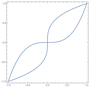
From your code I take it, you want to calculate the zeros of the function "f", what is not the same as the "basin of attraction", see below.

To get an idea about the zeros, we first make a contour plot of the 2 components of f:

f[{x_, y_}] = {x^3 - y, y^3 - x};

enter image description here

We have 3 zeros: {1,1}, {0,0}, {-1,-1}

To which zero the Newton method will take us depends on the starting point.

We first define a function that gives us a zero belonging to some start point:

  zero[fun_, start_] := Module[{invjacobian, pos = start, x, y},
  invjacobian[{x_, y_}] = Inverse[D[fun[{x, y}], {{x, y}}]];
  While[Norm[f[pos]] > 10^-6 , 
   pos = pos - invjacobian[pos] . f[pos]];
  pos]

We can try this e.g.:

zero[f, {0.5, 0.5}]

{-1., -1.}

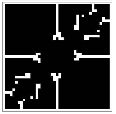
However, the Newton method can diverge. E.g. with zero[f, {1, 0}] the While command will never stop. We can exploit this to get an idea about the basin of attraction. For this we change the function "zero" to check if it diverges and return a "1" if it does and a "0" otherwise. With this we get:

zero1[fun_, start_] := 
 Module[{invjacobian, pos = start, x, y}, 
  invjacobian[{x_, y_}] = Inverse[D[fun[{x, y}], {{x, y}}]]; i = 0;
  While[Norm[f[pos]] > 10^-5 && Norm[pos] < 1000 , 
   pos = pos - invjacobian[pos] . f[pos]];
  If[Norm[pos] < 1000, 1, 0] ]

To get an idea about the basin of attraction we apply zero1 to a grid of starting points and visualize the output by an ArrayPlot:

basin = Table[zero1[f, #] & [{x, y}], {x, -2, 2, 0.1}, {y, -2, 2, 0.1}];
ArrayPlot[basin]

enter image description here

The basin of attraction is quite complicated.

$\endgroup$

Your Answer

By clicking “Post Your Answer”, you agree to our terms of service and acknowledge you have read our privacy policy.

Not the answer you're looking for? Browse other questions tagged or ask your own question.