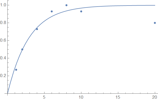
I want to fit the following equation
$\dot{B} ( t ) = \kappa ( 1 - B ( t ) ),$
to the dataset: $\{ ( 1.17, 0.27 ), ( 2, 0.5 ), ( 4, 0.73 ), ( 6, 0.93 ), ( 8, 1 ), ( 10, 0.93 ), ( 20, 0.8 ) \}$, where the first component is $t$ and the second $B$.
I'm using the following code for fitting:
Clear[fitness]

Bdata = {{1.17, 0.27}, {2, 0.5}, {4, 0.73}, {6, 0.93}, {8, 1}, {10, 0.93}, {20, 0.8}};
tk = {1.17, 2, 4, 6, 8, 10, 20};
y = {0.27, 0.5, 0.73, 0.93, 1, 0.93, 0.8};

fitness[kappa_?NumberQ, b0_?NumberQ] :=
Module[{bb, ode, ODE, solode, cinit, t},
ode = kappa (1 - bb[t]);
cinit = bb[0] == b0;
ODE = Join[ode, cinit];
solode = Quiet@NDSolve[ODE, bb, {t, tk[[1]], tk[[7]]}][[1]];
Return[
Sum[Norm[y[[k]] - Evaluate[bb[t] /. solode /. {t -> tk[[k]]}]], {k,
  1, 7}]]]

restrs = {0.1 < kappa < 0.9 && 0.1 < b0 < 1};
vars = {kappa, b0};

sol = Quiet@
FindMinimum[
Join[{fitness[kappa, b0]}, restrs], {{kappa, 0.15}, {b0, 0.15}},
StepMonitor :> Print[{kappa, b0, fitness[kappa, b0]}],
MaxIterations -> 10, WorkingPrecision -> 30]

ode = kappa (1 - bb[t]) /. sol[[2]];
cinit = bb[0] == b0 /. sol[[2]];
ODE = Join[ode, cinit];
solode = NDSolve[ODE, bb, {t, tk[[1]], tk[[7]]}][[1]];

plotb1 = Plot[Evaluate[bb[t] /. solode], {t, tk[[1]], tk[[7]]}];
plotb2 =
ListPlot[Transpose[{tk, y}], PlotStyle -> Blue, PlotLabel -> "B(t)"];
Show[plotb1, plotb2]
however, it returns many errors. Any help is appreciated for fixing the issues.
P.S. In principle, it is possible to solve the differential equation analytically, and then to use its solution for fitting, using NonlinearModelFit, but I'm interested to do fitting by directly using the ODE.

