0
$\begingroup$

I want to solve the following equation, and I want to get its analytical solution, but mathematica still can't give its analytical solution. Is there any way to make it give an analytical solution?

M = 1; Q = 0.7; a = 0.6; \[Alpha] = 0.9; l0 = 0.2;
Solve[r^2 - 2 M r - \[Alpha] l0 r + Q^2 - \[Alpha] M r Exp[-r/M] + 
   a^2 == 0, r]

Or is there any way to obtain its approximate analytical solution?

$\endgroup$
4
  • 3
    $\begingroup$ Few equations in mathematics have analytical solutions. $\endgroup$
    – John Doty
    Commented Jul 4, 2023 at 15:57
  • $\begingroup$ Is the result of Solve[r^2 - 2 M r - \[Alpha] l0 r + Q^2 - \[Alpha] M r Exp[-r/M] + a^2 == 0, r, Reals] satisfactory? (Tip: For exact solvers like Solve, it is usually better to use exact input. Floating-point numbers are treated as approximate. Numerical solvers like NSolve or FindRoot may be better choices if approximate results are desired or satisfactory.) $\endgroup$
    – Michael E2
    Commented Jul 4, 2023 at 16:11
  • $\begingroup$ Alternatively, one can find solutions in a bounded rectangle in $\Bbb C$ like this: NSolve[r^2 - 2 M r - \[Alpha] l0 r + Q^2 - \[Alpha] M r Exp[-r/M] + a^2 == 0 && -20 < Im[r] < 20 && -10 < Re[r] < 10, r]. It appears there may be infinitely many solutions without periodicity or other pattern that allows Mma to express the complete solution. Or: Solve[Rationalize[ 2 M r - \[Alpha] l0 r + Q^2 - \[Alpha] M r Exp[-r/M] + a^2 == 0] && -20 < Im[r] < 20 && -10 < Re[r] < 10, r] for exact Root[] objects. $\endgroup$
    – Michael E2
    Commented Jul 4, 2023 at 16:16
  • $\begingroup$ I think no chance. $\endgroup$
    – user64494
    Commented Jul 4, 2023 at 17:11

2 Answers 2

2
$\begingroup$
Clear["Global`*"]

M = 1; Q = 7/10; a = 3/5; α = 9/10; l0 = 1/5;

Restrict the domain to Reals

eqn = r^2 - 2 M r - α l0 r + Q^2 - α M r Exp[-r/M] + a^2 == 0;

sol = Solve[eqn, r, Reals]

enter image description here

Verifying the solutions,

eqn /. sol // FullSimplify

(* {True, True} *)

The result is given in terms of Root expressions. The approximate numeric values are

sol // N

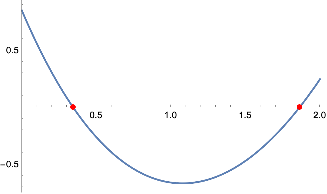
(* {{r -> 0.343441}, {r -> 1.86348}} *)

Graphically,

Plot[Evaluate@eqn[[1]], {r, 0, 2},
 Epilog -> {Red, AbsolutePointSize[6],
   Point[{r, 0} /. sol]}]

enter image description here

$\endgroup$
6
  • $\begingroup$ In fact, your sol is {{r -> Root[{-90*#1 + E^#1*(85 - 218*#1 + 100*#1^2) & , 0.3434410417590972717226381966222565957320.602059991322722}]}, {r -> Root[{-90*#1 + E^#1*(85 - 218*#1 + 100*#1^2) & , 1.8634831470915269008646784833389820068620.30103248076972}]}}. This is not any analytical solution. $\endgroup$
    – user64494
    Commented Jul 4, 2023 at 17:10
  • 1
    $\begingroup$ @user64494 - Root is as much of an analytic solution as any other higher transcendental function. The fact that is newer doesn’t make it any less useful. $\endgroup$
    – Bob Hanlon
    Commented Jul 4, 2023 at 17:20
  • $\begingroup$ The documentation says "Root represents an exact number as a solution to an equation f[x]==0 with additional information specifying which of the roots is intended", no more and no less. Also see Wiki for the definition of an analytical expression. $\endgroup$
    – user64494
    Commented Jul 4, 2023 at 17:29
  • 1
    $\begingroup$ @user64494 - from your link, “ However, the class of expressions considered to be analytic expressions tends to be wider than that for closed-form expressions. In particular, special functions such as the Bessel functions and the gamma function are usually allowed, and often so are infinite series and continued fractions.” Root is a newer special function. An exact value is what is required by many. $\endgroup$
    – Bob Hanlon
    Commented Jul 4, 2023 at 17:49
  • 1
    $\begingroup$ @user64494 For practical purposes, Root objects are about as good as more traditional analytic expressions. So, if your intent is to obstruct the solution of problems, you reject them, while if your intent is to enable the solution of problems you embrace them. $\endgroup$
    – John Doty
    Commented Jul 5, 2023 at 14:23
2
$\begingroup$

If the smaller solution is what you want, you could develop the exponential into a series like

Series[E^(-(r/M)), {r, 0, 3}]

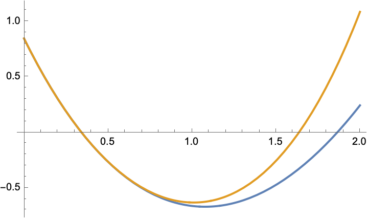
Higher order means better precision, but more complicated expressions... A plot shows the effect of the approximation:

M = 1; Q = 0.7; a = 0.6; \[Alpha] = 0.9; l0 = 0.2; 
Plot[{r^2 - 2*M*r - \[Alpha]*l0*r + Q^2 - \[Alpha]*M*r*Exp[-r/M] + 
a^2, a^2 + Q^2 - 2*M*r + r^2 - 
l0*r*\[Alpha] - (1 - r/M + r^2/(2*M^2) - r^3/(6*M^3))*M*
r*\[Alpha]}, {r, 0, 2}]

enter image description here

The equation using the approximation may then be solved analytically:

Solve[a^2 + Q^2 - 2*M*r + r^2 - 
l0*r*\[Alpha] - (1 - r/M + r^2/(2*M^2) - r^3/(6*M^3))*M*
r*\[Alpha] == 0, r]
(* lengthy expressions *)

As this is of 4th order you get 4 solutions. Here the third gives the zero around 0.34.

$\endgroup$
4
  • $\begingroup$ Think of Series[Exp[-r/M],{r,0,7}]//Normal instead of your Series[Exp[-r/M],{r,0,3}]//Normal, when there is no analytical solution . $\endgroup$
    – user64494
    Commented Jul 4, 2023 at 18:00
  • $\begingroup$ @user64494 but 4th order is the highest you can solve $\endgroup$
    – Andreas
    Commented Jul 4, 2023 at 18:04
  • $\begingroup$ "A plot shows the effect of the approximation" - better no say! In fact, you analytically solve a different equation than in the question. $\endgroup$
    – user64494
    Commented Jul 4, 2023 at 18:25
  • 1
    $\begingroup$ @user64494 the plot shows that in the area of interest both equations look similar. $\endgroup$
    – Andreas
    Commented Jul 5, 2023 at 8:41

Your Answer

By clicking “Post Your Answer”, you agree to our terms of service and acknowledge you have read our privacy policy.

Not the answer you're looking for? Browse other questions tagged or ask your own question.