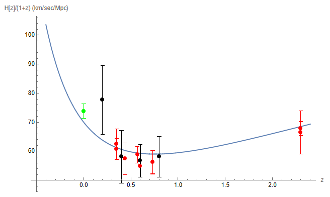
Maybe like this:
H0 = 70;
\[CapitalOmega]\[CapitalLambda] = 0.73;
\[CapitalOmega]M = 0.27;
H[z_] := H0*(\[CapitalOmega]\[CapitalLambda] + \[CapitalOmega]M*(1 +
     z)^3 + (1 - \[CapitalOmega]\[CapitalLambda] -
 \[CapitalOmega]M)*(1 + z)^2)^(1/2)

data0 = {{2.3, Around[66.5, 7.4]}, {2.3, Around[67.8, 2.4]}, {0.35,
Around[60.8, 3.6]}, {0.35, Around[62.5, 5.2]}, {0.57,
Around[58.8, 2.9]}, {0.44, Around[57.4, 5.4]}, {0.60,
Around[54.9, 3.8]}, {0.73, Around[56.2, 4.0]}};
data1 = {{0.2, Around[1.11, 0.17]*H0}, {0.4,
Around[0.83, 0.13]*H0}, {0.6, Around[0.81, 0.08]*H0}, {0.8,
Around[0.83, 0.1]*H0}};
data2 = {{0, Around[73.8, 2.5]}};

Show[{Plot[H[z]/(1 + z), {z, -0.4, 2.4}, AxesOrigin -> {-1/2, 50},
AxesLabel -> {z, "H[z]/(1+z) (km/sec/Mpc)"}, PlotRange -> All],
ListPlot[{data0, data1, data2}, PlotStyle -> {Red, Black, Green}]}]


ListPlotand overlay it with a standard Plot of your theoretical function. $\endgroup$I only took the data from Table 2 on page15 from paper. The two upvotes on this question, though, might say something negative about the site. $\endgroup$