Non Linear Oscillation Spring-Pendul

Question

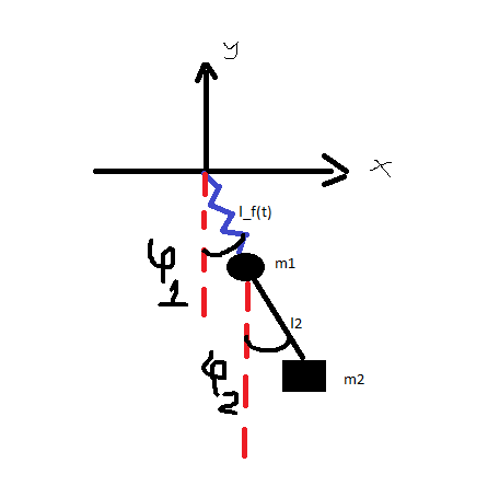
In a previews thread, I asked about how can I solve coupled PDEs. The problem I had was the following one:

What I was given were the following:

$\vec r_1(t)=l_f(t)(sin(\phi_1(t)),-cos(\phi_1(t)))$

$\vec r_2(t)=\vec r_1(t)+l_2(sin(\phi_2(t)),-cos(\phi_2(t)))$

l1 - was given as the rest position of the spring. With the help of a community member (Numerical solution for coupled PDEs) I was able to further develop and write down my code. But the problem is that, I forgot that here we are dealing with non-linear oscillation and I do not know how that should affect my expressions. And also the fact that the code doesn't work properly, I get errors, specially when I am trying to animate the whole process. This is how far I've gone:

x1[t_] = lf[t]*Sin[Phi1[t]]
y1[t_] = lf[t]*(-Cos[Phi1[t]])
x2[t_] = lf[t]*Sin[Phi1[t]] + l2*Sin[Phi2[t]]
y2[t_] = lf[t]*(-Cos[Phi1[t]]) - l2*Cos[Phi2[t]]

r1 = {x1[t], y1[t]}
r2 = {x2[t], y2[t]}

v1 = D[r1, t]
v2 = D[r2, t]

T = (1/2)*(m1*v1 . v1 + m2*v2 . v2);
U = m1*g*lf[t]*(1 - Cos[Phi1[t]]) + (1/2)*k1*(lf[t] - l1)^2 + 
  m2*g*(lf[t]*(1 - Cos[Phi1[t]]) + l2*(1 - Phi2[t]))

L = Simplify[T - U]

dLdPhi1 = D[L, Phi1[t]] // Simplify;
dLdPhiDot1 = D[L, Phi1'[t]] // Simplify;
ELEQ1 = dLdPhi1 == D[dLdPhiDot1, t];
ELEQ1 = Simplify[ELEQ1, {l1 != 0, m1 != 0, m2 != 0, l2 != 0, k1 != 0}]

dLdPhi2 = D[L, Phi2[t]] // Simplify;
dLdPhiDot2 = D[L, Phi2'[t]] // Simplify;
ELEQ2 = dLdPhi2 == D[dLdPhiDot2, t];
ELEQ2 = Simplify[ELEQ2, {l1 != 0, m1 != 0, m2 != 0, l2 != 0, k1 != 0}]

dLdlf = D[L, lf[t]] // Simplify;
dLdlfDot = D[L, lf'[t]] // Simplify;
ELEQ3 = dLdlf == D[dLdlfDot, t];
ELEQ3 = Simplify[ELEQ3, {l1 != 0, m1 != 0, m2 != 0, l2 != 0, k1 != 0}]

I am trying to make an animation out of it but I don't understand why the code is not running correctly:

Pendulum[{len1_, len2_, mass1_, mass2_, koef1_}, {
    lft_, Phi01_, Phi02_, lftdot_, Phi01dot_, Phi02dot_}] := Module[
    {gVal, tM, temp1, temp2, temp3, sol1, sol2, sol3, lfsol, phi1sol, 
   phi2sol, params, res},
    gVal = 9.81;
    tM = 60; (* timeMax *);
    (* Parameter einsetzen in Bewegungsgleichungen: *)
    params = {g -> gVal, len1 -> l1, len2 -> l2, mass1 -> m1, 
    mass2 -> m2, koef1 -> k1}; 
    temp1 = {ELEQ1} /. params; temp2 = {ELEQ2} /. params; 
  temp3 = {ELEQ3} /. params;
    (* Anfangsbedingungen hinzufuegen: *)
    temp1 = 
   Join[temp1, {Phi1[0] == Phi01, Phi1'[0] == Phi01dot, 
     Phi2[0] == Phi02, Phi2'[0] = Phi02dot, lf[0] = lft, 
     lf'[0] = lftdot}];
  temp2 = 
   Join[temp2, {Phi1[0] == Phi01, Phi1'[0] == Phi01dot, 
     Phi2[0] == Phi02, Phi2'[0] = Phi02dot, lf[0] = lft, 
     lf'[0] = lftdot}];
  temp3 = 
   Join[temp3, {Phi1[0] == Phi01, Phi1'[0] == Phi01dot, 
     Phi2[0] == Phi02, Phi2'[0] = Phi02dot, lf[0] = lft, 
     lf'[0] = lftdot}];
    (* DGL loesen und Fkt. definieren: *)
    sol1 = NDSolve[temp1, Phi1[t], {t, 0, tM}];
  sol2 = NDSolve[temp2, Phi2[t], {t, 0, tM}];
  sol3 = NDSolve[temp3, lf[t], {t, 0, tM}];
    phi1sol = Phi1[t] /. sol1[[1]];
  phi2sol = Phi2[t] /. sol2[[1]];
  lfsol = Phi2[t] /. sol3[[1]];
    (* Pendel animieren: *)
    res = 
   Animate[plotPendulum[phi1sol, phi2sol, lfsol /. {t -> tt}, tt, 
     params],
       {tt, 0, tM, 0.01 (* timeInt *)}];
    Return[res]
    ]

And here is the plotpendulum, which is the code that generates the picture that I painted:

plotPendulum[Phi1_, Phi2_, t_, subs_List ] := Module[
    {p1, p2, le, ps, ra, lines, dots, ceil, text, text2, all, 
   pendulum},
   
    p1 = {x1[t], y1[t]} /. subs;
    p2 = {x2[t], y2[t]} /. subs;
    
    le = (l1 + l2) /. subs;
  
    ra = le*{{-1.05, 1.05}, {-2.15, 2.15}};
    
    ceil  = {Brown, Thickness[0.05], 
    Line[{{-l, 0} /. subs, {l, 0} /. subs}]};
    lines = {Black, Thickness[0.01], Line[{{0, 0}, p1}], 
    Thickness[0.005], Line[{p1, p2}]};
    dots  = {Black, PointSize[0.04], Point[{{0, 0}, p1}], Red, 
    PointSize[0.1], Point[{p2}]};
  
    text = {Black, Background -> White,
        Text[m, p2 + {1, 0}, {-1, 0}],
        Text[l, p1 + (p2 - p1)/2 - {0.05*le, 0}, {1, 0}],
        Text[" t = " <> ToString[t] <> " s ", {-l*0.5, a} /. subs]};
    
    all = Join[ceil, lines, dots, text];
    pendulum = Show[Graphics[all], PlotRange -> ra];
    Return[pendulum]
    ]

When I try to execute the code: Pendulum[{1, 1, 1, 2, 100}, {0.9, 1/10, -5*Pi/4, 0, 0, 0}], I get errors of the kind:

NDSolve:Equation or list of equations expected instead of 0 in the first
argument

General::stop: Further output of NDSolve::deqn will be suppressed during this calculation.

Replaceall: is neither a list of replacement rules nor a valid dispatch table,
and so cannot be used for replacing.

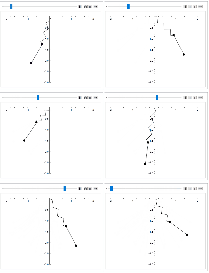
And the animation is blank

Answer 1

I do not enjoy debugging complicate programs. Instead I show a method that gives the result with much less effort.

Newtons method is easy to graps. However, for a lot of problems it gets very fast very complicated. The problem is, that by changing coordinates, Newtons formula is not conserved and can get quit complicated. That is why one introduced Lagrange's method. The Lagrange formula stays the same for arbitrary coordinates.

For the Lagrange method one needs to calculate the kinetic: T and the potential: V energy and take the difference: L= T-V, called the Lagrange function. The formula is then for every arbitrary coordinate: q, used to write L:

D[D[L,q'],t] - D[L,q] == 0

For a definitive example we need some constants and we choose a coordinate system with x to the right and y up.:

Clear["Global`*"]
m1 = 1; (*mass 1*)
m2 = 1;(*mass 2*)
k = 100;(*force constant of spring*)
l0 = 1;(*itial spring length*)
l2 = 1;(*length of rot of m2*)
g = 9.81(*earth acceleration*);

Then we calculate the positions of mass 1 and 2:

r1[t_] = l[t] { Sin[phi1[t]], -Cos[phi1[t]]};
r2[t_] =  r1[t] + l2 {Sin[phi2[t]], -Cos[phi2[t]]};

Now comes Lagrange into play. For this

V = 1/2  k (l[t] - l0)^ 2 + r1[t][[2]] m1 g + r2[t][[2]] m2 g;
T = 1/2 m1 r1'[t] . r1'[t] + 1/2 m2 r2'[t] . r2'[t];
L = T - V // Simplify;

Now the Lagrange equations:

eq = D[D[L, {{l'[t], phi1'[t], phi2'[t]}}], t] - 
      D[L, {{l[t], phi1[t], phi2[t]}}] == 0 // Simplify // Thread;

with the initial conditions:

ini = {l[0] == l0, phi1[0] == 1, phi2[0] == 1, l'[0] == 0, phi1'[0] == 0, phi2'[0] == 0};

we can solve:

sol = {l, phi1, phi2} /. NDSolve[Join[eq, ini], {l, phi1, phi2}, {t, 0, 10}][[1]];

Finally we may use the solution to draw a graphics:

spring[l0_?NumericQ, phi_] := 
  Module[{n = 5, d, w = 0.1, sp, t},
   d = l0/(n + 1);
   sp = Flatten[Table[{{w, -i d}, {-w, -(i + 1) d}}, {i, .5, n, 2}], 
     1];
   sp = Join[{{0, 0}}, sp, {{0, -l0}}];
   sp = RotationMatrix[phi] . # & /@ sp;
   {Line[sp], Disk[sp[[-1]], 0.05]}
   ];


Animate[
 (s = spring[sol[[1]][t], sol[[2]][t]];
  r1 = s[[-1, 1]];
  r2 = r1 + l2 {Sin[sol[[3]][t]], -Cos[sol[[3]][t]]};
  Graphics[{s, Line[{r1, r2}], Disk[r2, 0.05]}, 
   PlotRange -> {{-2, 2}, {-3, 0}}, Axes -> True])
 , {t, 0, 10}]