Fitting a two-dimensional Gaussian to a set of 2D pixels

Question

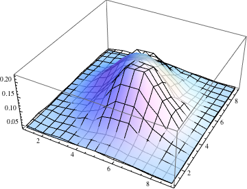
Imagine I have a set of data like the following:

data = {{0.0453803, 0.0427863, 0.0489815, 0.045243, 0.0488289, 0.0432898, 
  0.04448, 0.0387732, 0.0388952}, {0.0507668, 0.0427863, 0.0502632, 
  0.0503395, 0.0634623, 0.0675822, 0.0529335, 0.047425, 
  0.0387121}, {0.042237, 0.0501259, 0.0595712, 0.0869001, 0.139559, 
  0.141512, 0.0868391, 0.0579232, 0.0408331}, {0.0478981, 0.0491646, 
  0.0652628, 0.130404, 0.218448, 0.220645, 0.143603, 0.0605173, 
  0.0424964}, {0.0462043, 0.0530861, 0.076051, 0.140017, 0.206943, 
  0.202502, 0.118791, 0.0614023, 0.0459907}, {0.0511788, 0.0582132, 
  0.105531, 0.166354, 0.181003, 0.13698, 0.0748302, 0.0557107, 
  0.0492103}, {0.0493629, 0.0539712, 0.0971695, 0.160769, 0.164477, 
  0.104768, 0.0591745, 0.0475319, 0.0452583}, {0.0510719, 0.0599374, 
  0.0730602, 0.0975814, 0.101289, 0.0691997, 0.0498054, 0.044892, 
  0.043122}, {0.0460517, 0.0567025, 0.0574044, 0.0587778, 0.0537118, 
  0.0487221, 0.0474098, 0.0413977, 0.04477}}

How might I best fit a Gaussian curve to this set of datapoints, and extract properties such at the fit' semi-axes? I noticed that ComponentMeasurements has some functionality for best fit ellipsoids, but that doesn't seem to be workable here.

My objective here is to determine how "Gaussian" a set of points in an image are. My strategy is to sequentially fit a 2D Gaussian to each point, and then to measure it's eccentricity and spread (looking, for example, at the length and ratio of the semiaxes of the ellipsoid corresponding to the fit). The example here seems like it should yield a 2D Gaussian fit with significant spread and a ratio for the semiaxes significantly diverging from one.

Answer 1

Sjoerd's answer applies the power of Mathematica's very general model fitting tools. Here's a more low-tech solution.

If you want to fit a Gaussian distribution to a dataset, you can just find its mean and covariance matrix, and the Gaussian you want is the one with the same parameters. For Gaussians this is actually the optimal fit in the sense of being the maximum likelihood estimator -- for other distributions this may not work equally well, so there you will want NonlinearModelFit.

One wrinkle is that your data doesn't fall off to zero but to something like Min[data] $\approx 0.0387$, but we can easily get rid of that by just subtracting it off. Next, I normalize the array to sum to $1$, so that I can treat it like a discrete probability distribution. (All this really does is allow me to avoid dividing by Total[data, Infinity] every time in the following.)

min = Min[data];
sum = Total[data - min, Infinity];
p = (data - min)/sum;

Now we find the mean and covariance. Mathematica's functions don't seem to work with weighted data, so we'll just roll our own.

{m, n} = Dimensions[p];
mean = Sum[{i, j} p[[i, j]], {i, 1, m}, {j, 1, n}];
cov = Sum[Outer[Times, {i, j} - mean, {i, j} - mean] p[[i, j]], {i, 1, m}, {j, 1, m}];

We can easily get the probability distribution for the Gaussian with this mean and covariance. Of course, if we want to match the original data, we have to rescale and shift it back.

f[i_, j_] := PDF[MultinormalDistribution[mean, cov], {i, j}] // Evaluate;
g[i_, j_] := f[i, j] sum + min;

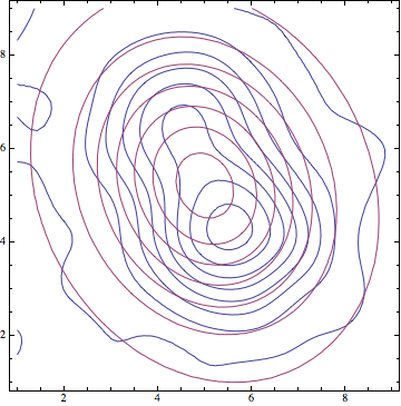
The match is not too bad, although the data has two humps where the Gaussian has one. You can also compare the fit through a contour plot. (Use the tooltips to compare contour levels.)

Show[ListPlot3D[data, PlotStyle -> None], 
 Plot3D[g[i, j], {j, 1, 9}, {i, 1, 9}, MeshStyle -> None, 
  PlotStyle -> Opacity[0.8]], PlotRange -> All]
Show[ListContourPlot[data, Contours -> Range[0.05, 0.25, 0.025], 
  ContourShading -> None, ContourStyle -> ColorData[1, 1], InterpolationOrder -> 3], 
 ContourPlot[g[i, j], {j, 1, 9}, {i, 1, 9}, Contours -> Range[0.05, 0.25, 0.025], 
  ContourShading -> None, ContourStyle -> ColorData[1, 2]]]

The variances along the principal axes are the eigenvalues of the covariance matrix, and the standard deviations (which I guess you're calling the semi-axes) are their square roots.

Sqrt@Eigenvalues[cov]
(* {1.86325, 1.50567} *)

Answer 2

data3D = Flatten[MapIndexed[{#2[[1]], #2[[2]], #1} &, data, {2}], 1];

fm = NonlinearModelFit[data3D, 
        a E^(-(((-my + y) Cos[b] - (-mx + x) Sin[b])^2/(2 sy^2)) - 
               ((-mx + x) Cos[b] + (-my + y) Sin[b])^2/(2 sx^2)), 
        {{a, 0.1}, {b, 0}, {mx, 4.5}, {my, 4.5}, {sx, 3}, {sy, 3}}, 
        {x, y}
     ]

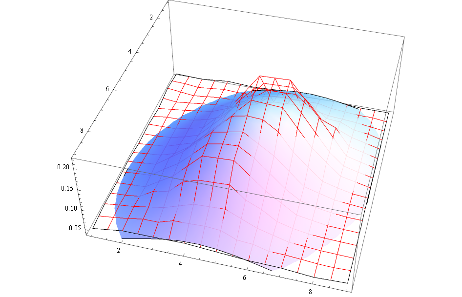
Show[
   ListPlot3D[data3D, PlotStyle -> None, MeshStyle -> Red],
   Plot3D[fm["BestFit"], {x, 1, 9}, {y, 1, 9}, PlotRange -> All, 
          PlotStyle -> Opacity[0.9], Mesh -> None]
]

fm["BestFitParameters"]

{a -> 0.1871830545, b -> -0.4853901689, mx -> 5.152549499, my -> 5.092511036, sx -> 2.756524919, sy -> 2.072163433}

Answer 3

Starting with your data, I would map out the data something like this:

data3D = Flatten[MapIndexed[{#2[[1]], #2[[2]], #1} &, data, {2}], 1]

and then count it like:

data2 = Flatten[Table[{#[[1]], #[[2]]}, {100 #[[3]]}] & /@ data3D, 1];

and then use this function:

FindDistributionParameters[data2, 
MultinormalDistribution[{a, b}, {{c, d}, {e, f}}]]

to find the means and coveriance of the data. And then I might do other stuff with the distribution, such as create a distribution object using:

edist = EstimatedDistribution[data2, 
MultinormalDistribution[{a, b}, {{c, d}, {e, f}}]]

and then check the distribution against the data, using:

dtest = DistributionFitTest[data2, edist, "HypothesisTestData"]

and create a table of the test results, using:

N[dtest["TestDataTable", All]]

or individually

AndersonDarlingTest[data2, edist, "TestConclusion"]
CramerVonMisesTest[data2, edist, "TestConclusion"]
JarqueBeraALMTest[data2, "TestConclusion"]
MardiaKurtosisTest[data2, "TestConclusion"]
MardiaSkewnessTest[data2, "TestConclusion"]
PearsonChiSquareTest[data2, edist, "TestConclusion"]
ShapiroWilkTest[data2, "TestConclusion"]

Now, I'm not a statistician, and I probably only know enough statistics to be dangerous, and I'm not familar with all the tests listed in the table, but I suspect that one of those small numbers is significant in measuring how close the actual data fits the distribution, i.e. how "Gaussian" the set of points is.

Also I might just plot the data as follows and visually judge the gaussiness of the data using these functions (as per VLC's answer to question 2984)

Show[DensityHistogram[d, {.2}, ColorFunction -> (Opacity[0] &), 
Method -> {"DistributionAxes" -> "Histogram"}], ListPlot[d]]

or these:

GraphicsColumn[
Table[SmoothDensityHistogram[d, ColorFunction -> "DarkRainbow", 
Method -> {"DistributionAxes" -> p}, ImageSize -> 500, 
BaseStyle -> {FontFamily -> "Helvetica"}, 
LabelStyle -> Bold], {p, {True, "SmoothHistogram", "BoxWhisker"}}]]

Answer 4

You mentioned in a related question that you would like to do large numbers of these fits quickly.

If each data set has the same dimensions, you can write a fairly fast implementation of Rahul Narain's method by precomputing arrays of x and y coordinates for the data grid, and flattening the data and using Dot to calculate the mean and the elements of the covariance matrix:

x = Table[i, {i, 9}, {j, 9}]//N;
y = Transpose[x];
x = Flatten[x]; y = Flatten[y];

semiaxes[data_] := Module[{min, p, mx, my},
  min = Min[data];
  p = Flatten[data] - min;
  p /= Total[p];
  mx = x.p;
  my = y.p;
  With[{a = (x - mx)^2.p, b = ((x - mx) (y - my)).p, c = (y - my)^2.p},
   Sqrt @ Eigenvalues[{{a, b}, {b, c}}]]]

semiaxes[data]
(* {1.86325, 1.50567} *)

This runs in about 340 µs on my PC

Compiling can give you even more speed, but you need to replace Eigenvalues with the explicit symbolic expressions:

semiaxesc = 
  With[{x = x, y = y}, 
   Compile[{{data, _Real, 2}}, Block[{min, p, mx, my, a, b, c},
     min = Min[data];
     p = Flatten[data] - min;
     p /= Total[p];
     mx = x.p;
     my = y.p;
     a = (x - mx)^2.p;
     b = ((x - mx) (y - my)).p;
     c = (y - my)^2.p;
      {Sqrt[1/2 (a + c - Sqrt[a^2 + 4 b^2 - 2 a c + c^2])],
       Sqrt[1/2 (a + c + Sqrt[a^2 + 4 b^2 - 2 a c + c^2])]}], 
    CompilationTarget -> "C", RuntimeOptions -> "Speed"]];

semiaxesc[data]
(* {1.50567, 1.86325} *)

This runs in about 5.7 µs on my PC.