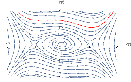
You do not need to solve the odes's to plot the solutions.
Let your first state variable be $x_1=x$ and the second be $x_2=y$. Then your odes are
\begin{align*}
x_1' &= x_2 \\
x_2' &= -x_1 +x_1^3 - 0.2 x_2
\end{align*}
Therefore the command in Mathematica to plot the solution is
StreamPlot[{x2, -x1 + x1^3 - 0.2*x2}, {x1, -2, 2}, {x2, -2, 2},
 Frame -> False, Axes -> True, AspectRatio -> 1/GoldenRatio,
 AxesLabel -> {"x(t)", "y(t)"},
 StreamPoints -> {{{{1, 1}, Red}, Automatic}},
 StreamColorFunction -> None]

The red line shows the solution for initial conditions $(1,1)$. Change as needed.
How can I plot X(t) vs t and y(t) vs t in 2 separate graphs?
You can do
s = NDSolveValue[{x'[t] == y[t], y'[t] == -x[t] + x[t]^3 - 0.2*y[t],
   x[0] == 0, y[0] == 1}, {x, y}, {t, 0, 3}]

opts = {GridLines -> Automatic, GridLinesStyle -> LightGray, ImageSize -> 300};
p1 = Plot[s[[1]][t], {t, 0, 3}, AxesLabel -> {"time (sec)", "x(t)"}, Evaluate@opts];
p2 = Plot[s[[2]][t], {t, 0, 3}, AxesLabel -> {"time (sec)", "y(t)"}, Evaluate@opts];
Grid[{{p1, p2}}, Frame -> All, Spacings -> {1, 1}]


{x[0],y[0]}={0,0}, the result is a segment on x-axis. Maybe change to{x[0],y[0]}={1,1}for example. $\endgroup${}button above the edit window. The edit window help button?is useful for learning how to format your questions and answers. You may also find the meta Q&A, How to copy code from Mathematica so it looks good on this site, helpful $\endgroup$