How to define the density of random 3D points and plot it?

Question

The following code draws a random distribution of particles in 3D. The Manipulate box allows to change a few parameters (number of particles, size of clusters, ...). I would like to define the local number of particles per unit volume $V = \ell^3$, on a variable scale $\ell$, and plot it as level curves (i.e surfaces) in 3D. How can this be done in Mathematica?

galaxies[p_, q_, r_] := Module[
    {pts = RandomReal[{-1, 1}, {p, 3}]},
    pts = Nest[Join[#, {RandomChoice[#] + r RandomReal[{-1, 1}, 3]}] &, pts, q];
    pts
]

graph[p_, q_, r_] := Graphics3D[{RGBColor[{0.5, 0.4, 1.0}], PointSize[0.004], Point[galaxies[p, q, r]]}]

view[p_, q_, r_] := Show[{graph[p, q, r]},
    PlotRange -> {{-1, 1}, {-1, 1}, {-1, 1}},
    Boxed -> True,
    Background -> Black,
    ImageSize -> {700, 700},
    SphericalRegion -> True,
    Method -> {"RotationControl" -> "Globe"}
]

Manipulate[
    view[p, q, r],
    {{p, 500, "Number of clusters"}, 1, 1000, 1},
    {{q, 10000, "Number of galaxies"}, 0, 10000, 1},
    {{r, 0.05, "Scale"}, 0, 0.2, 0.001},
    ControlPlacement -> Bottom
]

The scale $\ell$ should be a variable, from a small value up to the full box size, say : $0.01 \le \ell \le 2$, that could be changed in another Manipulate box. The idea is to plot the density of the particles in the box as a scalar function: $$\tag{1} \rho(x, y, z, \ell) = \frac{N(x, y, z, \ell)}{\ell^3}, $$ where $N(x, y, z, \ell)$ gives the total number of particles inside the cube of volume $V = \ell^3$, as a function of the cube center $\{x, y, z \}$ (with -1 < x, y, z < 1). I really don't know how to start to implement the idea, especially since the sampling volume should always stay inside the whole box of size $\ell_{max} = 2$ (with center located at $\{0, 0, 0 \}$). The sampling near the edges of the whole box may also be a problem (maybe the random distribution should be defined on a box two times larger than the display box).

EDIT: The exact "microscopic" density of the $N$ particles can be defined using Dirac's deltas: $$\tag{2} \rho(x, y, z) = \sum_{k \,=\, 1}^N \delta (x - x_k) \, \delta (y - y_k) \, \delta (z - z_k). $$ This density is 0 everywhere, except at the location of a particle. We could then introduce the averaged density on a volume $\ell^3$ (around a point of coordinates $\{x, y, z\}$), by integration: $$\tag{3} \bar{\rho}_{\ell}(x, y, z) = \frac{1}{\ell^3} \int_{x - \ell/2}^{x + \ell/2} \int_{y - \ell/2}^{y + \ell/2} \int_{z - \ell/2}^{z + \ell/2} \rho(x, y, z) \, dx \, dy \, dz. $$ That density could be called "fine grained" when $\ell$ is small, and "coarse grained" when $\ell$ is close to the size of the whole box. In all cases: $0.0001 \le \ell \le 2$ (since the random distribution above is enclosed in a box of size $2$).

I should have stated this already from the start in my question, sorry about that. The parameter $\ell$ should be a variable in a Manipulate box. The function (3) is what I would like to calculate for my random distribution (code above), and plot as a 3D graphics (level curves or surfaces?). Of course, we should get $\bar{\rho}_1(x, y, z) = N/8$ when $\ell = 2$.

Ideally, the density $\bar{\rho}_{\ell}(x, y, z)$ should be smoothed/interpolated to give some smooth level curves/surfaces in a plot, instead of ugly discontinuous jumps. So how should I do this, with Mathematica?

Answer 1

The following is an example based on a uniform distribution of points/galaxies, which can be adapted to any desired distribution. Also, some notes:

1. The code is given here only for educational purposes and several optimizations can be made.
2. Using Nearest[] is not the most efficient approach to calculate "counts in cells", ie the number of particles in growing spheres of radius $r$ around each galaxy. It is in fact rather inefficient.

First, let's make two populations of points

SeedRandom[12345]
data = RandomReal[{-2, 2}, {2000, 3}];
datarmin1 = Select[data, #.# <= 1 &];

For this approach (and all similar "counts in cells" methods), one needs either more overall galaxies (given by data) than then ones under study (given by datarmin1) or periodic boundary conditions (eg coming from an N-body sim).

Then we use Nearest[] to count the number $N(r)$ of points around each of the galaxies under study, within the larger sample:

r0 = 0.01;
rmax = 1.01;
dr = 0.05;
j`j = 0; SetSharedVariable[j`j];
ProgressIndicator[Dynamic[j`j], {0, (rmax - r0)/dr + 1}]
avNr = ParallelTable[{{r,N[Mean[Table[Length[Nearest[data, datarmin1[[i]], {Infinity, r}]], {i, 1,Length[datarmin1]}]]]}, j`j++;}[[1]], {r, 0.01, 1.01, 0.05},DistributedContexts -> Automatic] // AbsoluteTiming

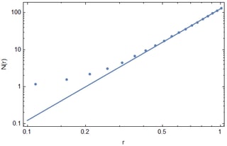
Then, one may fit this to a power-law, ie $N(r)\sim r^D$ and determine that indeed a uniform distribution of galaxies has a fractal dimension of D=3:

ff = FindFit[avNr[[2]], a r^D2, {a, D2}, r]

and a plot of the result:

The code can be adjusted for other distributions, as the one given by the OP (which will have a different fractal dimension).

Answer 2

Here is an approach that I hope gets after your objective of

I would like to define the local number of particles per unit volume V=ℓ3, on a variable scale ℓ, and plot it as level curves (i.e surfaces) in 3D.

(* Generate a universe *)
SeedRandom[12345];
galaxies[p_, q_, r_] := Module[{pts = RandomReal[{-1, 1}, {p, 3}]}, 
  pts = Nest[Join[#, {RandomChoice[#] + r RandomReal[{-1, 1}, 3]}] &, pts, q];
  pts]
universe = galaxies[500, 10000, 0.05];

(* Number of cells in each dimension of a n x n x n grid to hold densities *)
n = 101;
(* Set a size of cube for the calculation of density *)
(* Galaxies within s in each dimension are included for the
   calculation of density for each grid cell *)
s = 0.05;
(* Array to hold the densities *)
d = ConstantArray[0, {n, n, n}];
(* Add each galaxy to the cells within s of each galaxy location *)
Do[{x, y, z} = universe[[i]];
 ix0 = Max[1, Ceiling[1/2 (1 + n - (x - s) + n (x - s))]]; 
 ix1 = Min[n, Floor[(1 + n - (x + s) + n (x + s))/2]];
 iy0 = Max[1, Ceiling[1/2 (1 + n - (y - s) + n (y - s))]]; 
 iy1 = Min[n, Floor[(1 + n - (y + s) + n (y + s))/2]];
 iz0 = Max[1, Ceiling[1/2 (1 + n - (z - s) + n (z - s))]]; 
 iz1 = Min[n, Floor[(1 + n - (z + s) + n (z + s))/2]];
 Do[Do[Do[
    d[[ix, iy, iz]] = d[[ix, iy, iz]] + 1/(2 s)^3, {ix, ix0, ix1}], {iy, iy0, iy1}], {iz, iz0, iz1}],
 {i, Length[universe]}]

(* Create array to hold coordinates and density for cell in d *)
(* This is for the required input format to ListContourPlot3D *)
density = ConstantArray[{0, 0, 0, 0}, n^3];
m = 0;
(* Convert cell indices to locations and add to the density array *)
Do[x = (-1 + 2 i - n)/(-1 + n); 
 Do[y = (-1 + 2 j - n)/(-1 + n); 
  Do[z = (-1 + 2 k - n)/(-1 + n);
   m = m + 1; 
   density[[m]] = {x, y, z, d[[i, j, k]]}, {i, n}], {j, n}], {k, n}]

(* Take a look at the resulting densities to consider *)
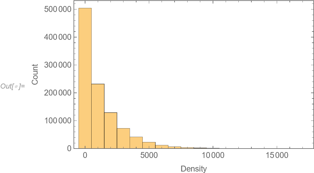
Histogram[density[[All, 4]], "FreedmanDiaconis", Frame -> True, 
 FrameLabel -> {"Density", "Count"}]

(* Choose a density of interest for contour *)
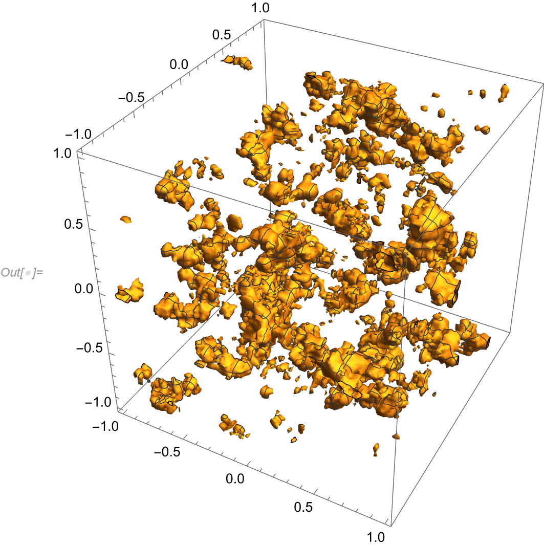
contourDensity = 5000;

(* ContourPlot3D *)
LBoxRatios -> {1, 1, 1}, MaxPlotPoints -> 100]

(* As a check on what is produced by ContourPlot3D, 
   show all of the grid points with a density of at least countourDensity *)
h = Select[density, #[[4]] > contourDensity &];
ListPointPlot3D[h[[All, {1, 2, 3}]], BoxRatios -> {1, 1, 1}]